Tutorial 1: An introduction to History Matching and Emulation, and the hmer package
1 Introduction
This short tutorial gives an overview of history matching with emulation and shows how to implement this technique in a one-dimensional example using the hmer package.
In this section, we introduce the concepts of history matching and emulation and explain how their combined use provides us with a way of calibrating complex computer models.
Computer models, otherwise known as simulators, have been widely used in almost all fields in science and technology. This includes the use of infectious disease models in epidemiology and public health. A computer model is a way of representing the fundamental dynamics of a system. Due to the complexity of the interactions within a system, computer models frequently contain large numbers of parameters.
Before using a model for projection or planning, it is fundamental to explore plausible values for its parameters, calibrating the model to the observed data. This poses a significant problem, considering that it may take several minutes or even hours for the evaluation of a single scenario of a complex model. This difficulty is compounded for stochastic models, where hundreds or thousands of realisations may be required for each scenario. As a consequence, a comprehensive analysis of the entire input space, requiring vast numbers of model evaluations, is often unfeasible. Emulation, combined with history matching, allows us to overcome this issue.
1.1 History Matching
History matching concerns the problem of identifying those parameter sets that may give rise to acceptable matches between the model outputs and the observed data. History matching proceeds as a series of iterations, called waves, where implausible areas of parameter space, i.e. areas that do not give rise to a match with the observed data, are identified and discarded. Each wave focuses the search for implausible space in the space that was characterized as non-implausible in all previous waves: thus the non-implausible space shrinks with each wave. To decide whether a parameter set \(x\) is implausible we introduce the implausibility measure, which evaluates the difference between the model results and the observed data, weighted by how uncertain we are at \(x\). If such measure is too high, the parameter set is discarded in the next wave of the process.
Note that history matching as just described still relies on the evaluation of the model at a large number of parameter sets, which is often unfeasible. Here is where emulators play a crucial role.
1.2 Emulators
A long established method for handling computationally expensive models is to first construct an emulator: a fast statistical approximation of the model that can be used as a surrogate. In other words, we can think of an emulator as a way of representing our beliefs about the behaviour of a complex model. Note that one can either construct an emulator for each of the model output separately, or combine outputs together, through more advanced techniques. From here on we assume that each model output will have its own emulator.
The model is run at a manageable number of parameter sets to provide training data for the emulator. The emulator is then built and can be used to obtain an expected value of the model output at any parameter set \(x\), along with a corresponding uncertainty estimate reflecting our beliefs about the uncertainty in the approximation.
Emulators have two useful properties. First, they are computationally efficient - typically several orders of magnitude faster than the computer models they approximate. Second, they allow for the uncertainty in their approximations to be taken into account. These two properties mean that emulators can be used to make inferences as a surrogate for the model itself. In particular, when going through the history matching process, it is possible to evaluate the implausibility measure at any given parameter set by comparing the observed data to the emulator output, rather than the model output. This greatly speeds up the process and allows for a comprehensive exploration of the input space.
1.3 History matching and emulation in a nutshell
Figure 1.1 shows a typical history matching workflow.
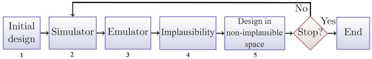
Figure 1.1: History matching and emulation flowchart
The various steps of the process can be summarised as follows:
- A number of parameter sets are selected.
- The model is run at the selected parameter sets.
- Emulators are built using the training data provided by the previous step. Note that here we initially choose to construct separate emulators, one for the mean of each model output, but more advanced approaches are possible.
- Emulators are evaluated at a large number of parameter sets. The implausibility of each of these is then assessed.
- Parameter sets classified as non-implausible will be used in the next wave of the process. From here, we go back to step 2).
Each time we get to step 5) we need to decide if to go for another wave or to stop the process. One stopping criterion consists in having all model runs at the current non-implausible space close enough to the targets: this means that we have fitted our model and we don’t need to perform another wave of history matching. In some other cases we might notice that the uncertainty of current emulators is smaller than the uncertainty in the targets: this implies that the non-implausible space is unlikely to decrease in size in the next wave and therefore it is best to stop the process. Finally we might end up with all the input space deemed implausible at the end of a wave. In this situation, we would deduce that there are no parameter sets that give an acceptable match with the data: in particular, this would raise doubts about the adequacy of the chosen model.
In the next section we give a very simple example of history matching and emulation to help the reader familiarise themselves with the procedure.