2 One-dimensional Example

To show how history matching and emulation work, we present a one-dimensional example, i.e. our model will have only one parameter. Our focus here is on the various steps of the process, rather than on the use of the hmer package. A more detailed introduction to the functionalities of hmer can be found in Tutorial 2.

2.1 Setup

The model we consider is a single univariate deterministic function:

\(f(x) = 2x + 3x\sin\left(\frac{5\pi(x-0.1)}{0.4}\right).\)

Through this very simple example we demonstrate the main features of emulation and history matching over a couple of waves. Moreover, since \(f(x)\) can be evaluated quickly, we will be able to compare the emulator performance against the actual function very easily.

func <- function(x) {
  2*x + 3*x*sin(5*pi*(x-0.1)/0.4)
}

We will presume that we want to emulate this function over the input range \(x\in[0,0.6]\). To train an emulator to this function, we’ll evaluate \(f\) at equally spaced-out points along the parameter range: \(10\) points will be ample for training a one-dimensional emulator.

data1d <- data.frame(x = seq(0.05, 0.5, by = 0.05), f = func(seq(0.05, 0.5, by = 0.05)))

For demonstration purposes we put no points between \(0.5\) and \(0.6\) in data1d: we will comment on the effects of this choice at the end of the first wave. Note that the value of \(f\) is considered unknown for all values of \(x\) outside data1d. The points in data1d will be passed to the hmer package, in order for it to train an emulator to the function func, interpolate points between the data points above, and propose a new set of points for training a second-wave emulator.

2.2 Emulator Training

To train the emulator, we first define the ranges of the parameters. Note that we create a list of one element, which seems pointless here but generalises easily to multi-output emulation.

ranges1d <- list(x = c(0, 0.6))

To build our emulator we use the function emulator_from_data, which requires at least three things: the training data data1d, the name(s) of the outputs to emulate, and the ranges of the input parameters ranges1d:

em1d_1 <- emulator_from_data(data1d, c('f'), ranges1d)

This trained emulator takes into account the fact that we know the values at the 10 points in the dataset. Correspondingly, the variance at these ten points (which we get through the get_cov method to em1d_1$f) is \(0\) and the expectation (which we get through the get_exp method to em1d_1$f) exactly matches the function value (up to numerical precision).

em1d_1$f$get_cov(data1d)
#>  [1] 0 0 0 0 0 0 0 0 0 0
em1d_1$f$get_exp(data1d) - data1d$f
#>  [1]  6.078471e-15 -7.771561e-16 -1.609823e-14 -2.908784e-14 -2.342571e-14
#>  [6] -1.532108e-14 -8.493206e-15 -8.770762e-15 -1.021405e-14 -5.551115e-15

We can use this trained emulator to predict the value at many points along the input range. Let’s define a large set of points to evaluate at, and get the emulator expectation and variance at each of these points.

test_points <- data.frame(x = seq(0, 0.6, by = 0.001))
em_exp <- em1d_1$f$get_exp(test_points)
em_var <- em1d_1$f$get_cov(test_points)

Because in this particular example the function to emulate is straightforward to evaluate, we will put all the test points into the actual function too. We create a data.frame with everything we need for plotting.

plotting1d <- data.frame(
  x = test_points$x,
  f = func(test_points$x),
  E = em_exp,
  max = em_exp + 3*sqrt(em_var),
  min = em_exp - 3*sqrt(em_var)
)

We now plot a set of items: the actual function (in black), the emulator expectation for the function (in blue), and \(3\sigma\) uncertainty bounds corresponding to the emulator variance (in red). We also plot the locations of the training points to demonstrate the vanishing variance at those points.

plot(data = plotting1d, f ~ x, ylim = c(min(plotting1d[,-1]), max(plotting1d[,-1])),
     type = 'l', main = "Emulation of a Simple 1-dimensional Function", xlab = "Parameter value", 
     ylab = "Function value")
lines(data = plotting1d, E ~ x, col = 'blue')
lines(data = plotting1d, min ~ x, col = 'red', lty = 2)
lines(data = plotting1d, max ~ x, col = 'red', lty = 2)
points(data = data1d, f ~ x, pch = 16, cex = 1)
legend('topleft', inset = c(0.05, 0.05), legend = c("Function value", "Emulated value", "Uncertainty Bounds"),
       col = c('black', 'blue', 'red'), lty = c(1,1,2))

We can note a few things from this plot. Firstly, the emulator does exactly replicate the function at the points used to train it (the black dots). The variance, i.e. the distance between the two red lines, increases the further away we get from a ‘known’ point, and indeed the emulator expectation starts to deviate from the actual function value. This is evident if we look at the area in between \(0.5\) and \(0.6\): since data1d contains no value in that interval, our emulator is particularly uncertain there. However, note that the actual value (the black line) never falls outside the \(3\sigma\) bounds given by the emulator variance.

2.3 History Matching

Now suppose that we want to find input points which result in a given output value. Obviously, with this function we can easily do this either analytically or numerically, but for complex models this is simply not possible. We therefore follow the history matching approach.

The first thing we need is a target value: let’s suppose we want to find points \(x\) such that \(f(x)=0\), plus or minus \(0.05\). Then we define our target as follows:

target1d <- list(f = list(val = 0, sigma = 0.05))

Again, the use of a list of lists is to ensure it generalises to multiple outputs.

We can now use the function generate_new_design to obtain a new set of points for the second wave. There are a multitude of different methods that can be used to propose the new points: in this particular one-dimensional case, it makes sense to take the most basic approach. This is to generate a large number of space-filling points, reject those that the emulator rules out as implausible, and select the subset of the remaining points that has the maximal minimum distance between them (so as to cover as much of the non-implausible space as possible). This can be done by setting method to lhs (Latin Hypercube sampling) and measure.method to maximin:

new_points1d <- generate_new_design(em1d_1, 10, target1d,
                                  method = 'lhs', 
                                  measure.method = 'maximin')

The output new_points1d consists of 10 points that were deemed non-implausible by the emulator em1d_1.

Having obtained these new points, let’s include them on our plot (blue dots) to demonstrate the emulator’s logic.

plot(data = plotting1d, f ~ x, ylim = c(min(plotting1d[,-1]), max(plotting1d[,-1])),
     type = 'l', main = "Emulation of a Simple 1-dimensional Function", xlab = "Parameter value", 
     ylab = "Function value")
lines(data = plotting1d, E ~ x, col = 'blue')
lines(data = plotting1d, min ~ x, col = 'red', lty = 2)
lines(data = plotting1d, max ~ x, col = 'red', lty = 2)
points(data = data1d, f ~ x, pch = 16, cex = 1)
legend('topleft', inset = c(0.05, 0.05), legend = c("Function value", "Emulated value", "Uncertainty Bounds"),
       col = c('black', 'blue', 'red'), lty = c(1,1,2))
abline(h = target1d$f$val, lty = 2)
abline(h = target1d$f$val + 3*target1d$f$sigma, lty = 2)
abline(h = target1d$f$val - 3*target1d$f$sigma, lty = 2)
points(x = unlist(new_points1d, use.names = F), y = func(unlist(new_points1d, use.names = F)), 
       pch = 16, col = 'blue')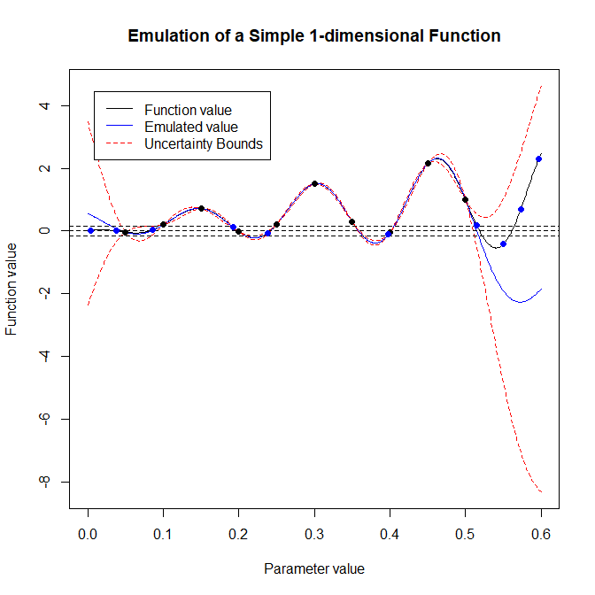

There is a crucial point here. While the emulator has proposed points that lie in the desired range (particularly on the left hand side of the interval), it has also proposed points that certainly do not lie in that range. However, at these points the range is contained within the band given by the emulator uncertainty bounds. Consider the right hand side of the interval: since the emulator has high variance there, it cannot rule out this region as unfeasible. This is the reason why generate_new_design proposes points there: in this way, when a new emulator will be trained in the second wave of the process, it will be much more certain about the function value than our current emulator in the interval \([0.5,0.6]\). This will allow the new emulator to rule out the area quickly.

2.4 Second Wave

The second wave is very similar to the first one: the model is evaluated at points in new_points1d and the outputs are used to train new emulators.

new_data1d <- data.frame(x = unlist(new_points1d, use.names = F), f = func(unlist(new_points1d, use.names = F)))

em1d_2 <- emulator_from_data(new_data1d, c('f'), ranges1d)
em1d_2_results <- data.frame(E = em1d_2[[1]]$get_exp(test_points), V = em1d_2[[1]]$get_cov(test_points))
plotting1d2 <- data.frame(x = plotting1d$x, f = plotting1d$f, E = em1d_2_results$E,
                          max = em1d_2_results$E + 3*sqrt(abs(em1d_2_results$V)),
                          min = em1d_2_results$E - 3*sqrt(abs(em1d_2_results$V)))
plot(data = plotting1d2, f ~ x,  ylim = c(min(plotting1d2[,-1]), max(plotting1d2[,-1])),
     type = 'l', main = "Emulator of a Simple 1-dimensional Function: Wave 2", xlab = "Parameter value", 
     ylab = "Function value")
lines(data = plotting1d2, E ~ x, col = 'blue')
lines(data = plotting1d2, max ~ x, col = 'red', lty = 2)
lines(data = plotting1d2, min ~ x, col = 'red', lty = 2)
points(data = new_data1d, f ~ x, pch = 16, cex = 1)
legend('topleft', inset = c(0.05, 0.05), legend = c("Function value", "Emulated value", "Uncertainty Bounds"), 
       col = c('black', 'blue', 'red'), lty = c(1,1,2))

This plot underlines the importance of using all waves of emulation. The first wave is trained over the entire space, and so gives a moderately confident estimate of the true function value on the interval \([0, 0.6]\). The second-wave emulator is trained only on regions that we need to be more certain of, i.e. on regions where the first-wave emulator was less certain. This is reflected for example on the fact that most points in new_data1d are above \(0.5\) or below \(0.1\). As a result, the second-wave emulator is much more certain than the first-wave emulator when \(x\) is above \(0.5\) or below \(0.1\). On the contrary, the second-wave emulator is particularly uncertain in the central region: this does not pose a problem, since the first-wave emulator was already approximating the model very well in that area. This is the reason why, when generating new non-implausible points at the end of the second wave, we must search for points with implausibility below three according to both the first- and the second-wave emulator:

new_new_points1d <-  generate_new_design(c(em1d_2, em1d_1), 10, z = c(target1d, target1d),
                                      method = 'lhs', measure.method = 'maximin')
plot(data = plotting1d2, f ~ x, ylim = c(min(plotting1d2[,-1]), max(plotting1d2[,-1])),
     type = 'l', main = "Emulator of a Simple 1-dimensional Function: Wave 2", xlab = "Parameter value", 
     ylab = "Function value")
lines(data = plotting1d2, E ~ x, col = 'blue')
lines(data = plotting1d2, max ~ x, col = 'red', lty = 2)
lines(data = plotting1d2, min ~ x, col = 'red', lty = 2)
points(data = new_data1d, f ~ x, pch = 16, cex = 1)
legend('topleft', inset = c(0.05, 0.05), legend = c("Function value", "Emulated value (wave 2)",
                                                    "Uncertainty Bounds"), col = c('black', 'blue', 'red'), 
                                                    lty = c(1,1,2))
abline(h = target1d$f$val, lty = 2)
abline(h = target1d$f$val + 3*target1d$f$sigma, lty = 2)
abline(h = target1d$f$val - 3*target1d$f$sigma, lty = 2)
points(x = unlist(new_new_points1d, use.names = F), y = func(unlist(new_new_points1d, use.names = F)), 
       pch = 16, col = 'blue')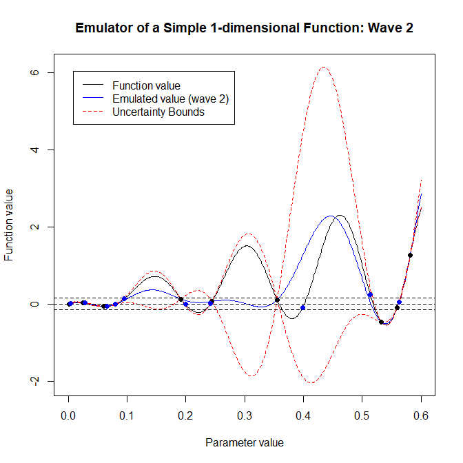

At the end of the second wave we see that all proposed points (in blue) are within the target bounds. For this reason we can end here the history matching process.