Tutorial 2: An introduction to the main functionalities of the hmer package
1 Introduction to the model
This tutorial presents the main functionalities of the hmer package, using a synthetic example of an epidemiological model. Although self-contained, this tutorial is the natural continuation of Tutorial 1, which gives an overview of the history matching with emulation process and shows how it works through a simple one-dimensional example. Readers who are not familiar with history matching and emulation will find Tutorial 1 particularly helpful.
Note that when running the workshop code on your device, you should not expect the hmer visualisation tools to produce the same exact output as the one you can find in the following sections. This is mainly because the maximinLHS function, that you will use to define the initial parameter sets on which emulators are trained, does return different Latin Hypercube designs at each call.
The model that we chose for demonstration purposes is a stochastic SEIRS model, with four parameters: rate of transmission between each infectious person and each susceptible person \(\beta_M\); transition rate from exposed to infectious \(\gamma_M\); recovery rate from infectious to recovered \(\delta_M\); and a ‘loss of immunity’ rate from recovered to susceptible \(\mu_M\).

Figure 1.1: SEIRS Diagram
Expressed in terms of differential equations, the transitions are \[\begin{align} \frac{dS}{dt} &= -\frac{\beta_M S I}{N} + \mu_M R \\ \\ \frac{dE}{dt} &= -\gamma_M E + \frac{\beta_M S I}{N} \\ \\ \frac{dI}{dt} &= -\delta_M I + \gamma_M E \\ \\ \frac{dR}{dt} &= -\mu_M R + \delta_M I \end{align}\] where \(N\) represents the total population, \(N=S+E+I+R\). For simplicity, we consider a closed population, so that \(N\) is constant.
To generate runs from this model, we use SimInf, a package that provides a framework to conduct data-driven epidemiological modelling in realistic large scale disease spread simulations. Note that the hmer package is code-agnostic: although we chose SimInf for this case study, hmer can be used to calibrate models written in any package or programming language. SimInf requires us to define the transitions, the compartments, and the initial population. If we want multiple repetitions for each choice of parameters, we create a data.frame with identical rows, each of which has the same initial population. Here we will choose \(50\) repetitions per choice of parameters and consider an initial population of \(1000\) of who \(50\) are infected. Note that if we were to start with one infectious individual, some runs of the model are likely not show an epidemic (since it could happen that the only infectious person recovers before infecting other people). Choosing a relatively high number of initial infectious people helps us circumvent any problems that would come from bimodality and keep the tutorial simple. Bimodality will be dealt in the more advanced case studies (see Stochastic Workshop.
compartments <- c("S","E","I","R")
transitions <- c(
  "S -> beta*I*S/(S+I+E+R) -> E",
  "E -> gamma*E -> I",
  "I -> delta*I -> R",
  "R -> mu*R -> S"
)
nreps <- 50
u0 <- data.frame(
  S = rep(950, nreps),
  E = rep(0, nreps),
  I = rep(50, nreps),
  R = rep(0, nreps)
)
We select parameter values and parse the model using the function mparse, which takes transitions, compartments, initial values of each compartment, parameter values and the time span to simulate a trajectory. We then run the model and plot the trajectories of interest.
params <- c(beta = 0.5, gamma = 0.5, delta = 0.1, mu = 0.1)
model <- mparse(transitions = transitions, compartments = compartments, u0 = u0, gdata = params, tspan = 1:60)
result = run(model)
plot(result)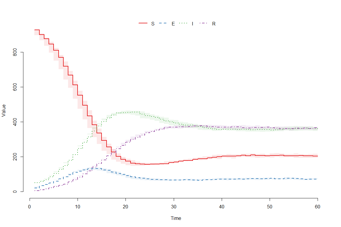
In order to extract the relevant information from the data provided by the SimInf run, a helper function getOutputs has been included in this document. It takes a data.frame of parameter sets and a list of times, and returns a data.frame of the results. We then create a data.frame outputs by binding the parameter values and the results obtained.
points <- expand.grid(list(beta = c(0.4, 0.6),
                           gamma = c(0.4, 0.6),
                           delta = c(0.05, 0.15),
                           mu = c(0.05, 0.15)
))
results <- getOutputs(points, seq(10,30,by=5))
outputs <- data.frame(cbind(points, results))
head(outputs)
#>   beta gamma delta   mu    I10    I15    I20    I25    I30     EV10     EV15
#> 1  0.4   0.4  0.05 0.05 221.50 405.46 543.52 571.92 537.30 5.698469 7.729000
#> 2  0.6   0.4  0.05 0.05 365.70 599.28 633.32 574.88 517.78 7.225607 5.610822
#> 3  0.4   0.6  0.05 0.05 279.72 490.88 595.46 580.54 534.48 7.260588 8.011528
#> 4  0.6   0.6  0.05 0.05 464.84 664.26 634.62 562.00 510.44 8.169654 4.577007
#> 5  0.4   0.4  0.15 0.05 108.94 164.18 210.14 225.46 216.06 4.977698 6.598832
#> 6  0.6   0.4  0.15 0.05 199.56 302.46 313.72 260.48 209.50 7.484863 7.184362
#>       EV20     EV25     EV30
#> 1 6.692455 4.506137 4.242956
#> 2 4.338955 4.974998 4.811440
#> 3 5.154793 4.252850 4.251787
#> 4 4.165780 4.501462 4.414445
#> 5 6.915291 5.450934 4.659115
#> 6 4.866044 4.805986 5.270938
Each row of outputs corresponds to a parameter set and contains information regarding the number of infectious individuals \(I\) for that set. Each row of column \(I10\) (resp. \(I15, I20, I25, I30\)) contains the mean value of \(I\) at time \(10\) (resp. \(15, 20, 25, 30\)) for the \(50\) runs of the relative parameter set. Similarly, columns \(EV10, EV15, EV20, EV25, EV30\) provide a measure of the
ensemble variability
for each parameter set, at each desired time: this is defined here as the standard deviation of the \(50\) runs, plus \(3\%\) of the range of the runs. The trained emulators outputs will be estimates of the means, while the ensemble variability will be used to quantify the uncertainty of such estimates.
Before we tackle the emulation, we need a set of wave0 data. For this, we define a set of ranges for the parameters, and generate parameter sets using a Latin Hypercube design (see fig. 1.2 for a Latin Hypercube example in two dimensions). We will run the model over \(80\) parameter sets; \(40\) of these will be used for training while the other \(40\) will form the validation set for the emulators.

Figure 1.2: An example of Latin hypercube in two dimensions: there is only one sample point in each row and each column.
Through the function maxminLHS we create two hypercube designs with 40 parameter sets each: one to train emulators and one to validate them.
ranges <- list(
  beta = c(0.2, 0.8),
  gamma = c(0.2, 1),
  delta = c(0.1, 0.5),
  mu = c(0.1, 0.5)
)
pts_train <- 2*(maximinLHS(40, 4)-1/2)
pts_valid <- 2*(maximinLHS(40, 4)-1/2)
r_centers <- map_dbl(ranges, ~(.[2]+.[1])/2)
r_scales <- map_dbl(ranges, ~(.[2]-.[1])/2)
pts_train <- data.frame(t(apply(pts_train, 1, function(x) x*r_scales + r_centers)))
pts_valid <- data.frame(t(apply(pts_valid, 1, function(x) x*r_scales + r_centers)))
pts <- rbind(pts_train, pts_valid)
head(pts)
#>        beta     gamma     delta        mu
#> 1 0.3466060 0.6188315 0.4233225 0.3962449
#> 2 0.6111659 0.3898439 0.3237638 0.2518652
#> 3 0.4870215 0.4251581 0.3344711 0.2259778
#> 4 0.4534464 0.6352057 0.2822131 0.1803356
#> 5 0.6827735 0.8566109 0.3444991 0.2132621
#> 6 0.3639475 0.3683167 0.2146582 0.1309577
Note that the first time we create pts_train (or pts_valid), we get \(40\) parameter sets where each parameter value is distributed on \([-1,1]\). This is not exactly what we need, since each parameter has a different range. We therefore define r_centers (resp. r_scales) which contains the midpoint (resp. the size) of the range of each parameter. Using these two pieces of information, we re-center and re-scale pts_train and pts_valid.
We obtain the model runs for the parameter sets in pts through the getOutputs function. We bind the parameter sets in pts to the model runs and save everything in the data.frame wave0.
wave0 <- data.frame(cbind(pts,getOutputs(pts, seq(10,30,by=5)))) %>%
setNames(c(names(ranges), paste0("I",seq(10,30,by=5)),paste0('EV',seq(10,30,by=5))))
head(wave0)
#>        beta     gamma     delta        mu    I10    I15    I20    I25    I30
#> 1 0.3466060 0.6188315 0.4233225 0.3962449  17.88  12.94   9.54   7.02   5.30
#> 2 0.6111659 0.3898439 0.3237638 0.2518652  72.08 105.60 130.40 145.56 151.32
#> 3 0.4870215 0.4251581 0.3344711 0.2259778  48.32  58.48  64.68  73.98  80.84
#> 4 0.4534464 0.6352057 0.2822131 0.1803356  69.38  90.08 104.14 116.30 123.18
#> 5 0.6827735 0.8566109 0.3444991 0.2132621 134.62 168.98 176.16 167.70 164.00
#> 6 0.3639475 0.3683167 0.2146582 0.1309577  58.22  72.34  91.18 105.00 114.32
#>       EV10     EV15     EV20     EV25     EV30
#> 1 2.259318 2.035119 1.330287 1.172772 1.180312
#> 2 4.088561 5.065905 4.982918 4.087230 4.676331
#> 3 2.982661 3.842215 4.201149 4.725206 4.871631
#> 4 4.693368 5.311363 5.924968 5.186154 5.342822
#> 5 6.414478 5.683270 3.922762 3.823964 4.053331
#> 6 3.542558 5.625714 5.534793 6.294237 5.562650
Finally, we split wave0 into two parts: the training set, on which we will train the emulators, and a validation set, which will be used to do diagnostics of the emulators.