4 Constructing the emulators

To construct the emulators, we use the function emulator_from_data, which requires at least the training data, the name of the model outputs to emulate and the list of parameter ranges. In this case study we also use the optional argument ev to pass our estimates of the ensemble variability. We first define the model output names and we calculate the ensemble variability evs taking the mean of the column \(EV\) in wave0:

output_names <- paste0("I", seq(10,30, by=5))
evs <- apply(wave0[10:ncol(wave0)], 2, mean)

The function emulator_from_data uses evs to estimate the delta parameter, i.e. the proportion of the overall variance due to the ensemble variability.

ems0 <- emulator_from_data(train0, output_names, ranges, ev=evs)
ems0[[1]]
#> Parameters and ranges:  beta: c(0.2, 0.8): gamma: c(0.2, 1): delta: c(0.1, 0.5): mu: c(0.1, 0.5) 
#> Specifications: 
#>   Basis functions:  (Intercept); beta; gamma; delta; mu; I(delta^2); beta:gamma; beta:delta; gamma:delta 
#>   Active variables beta; gamma; delta; mu 
#>   Regression Surface Expectation:  79.4188; 93.1408; 42.2031; -102.4974; 4.5401; 54.2205; 50.5944; -72.7635; -32.854 
#>   Regression surface Variance (eigenvalues):  0; 0; 0; 0; 0; 0; 0; 0; 0 
#> Correlation Structure: 
#> Bayes-adjusted emulator - prior specifications listed. 
#>   Variance (Representative):  251.1956 
#>   Expectation:  0 
#>   Correlation type: exp_sq 
#>   Hyperparameters:  theta: 0.8621 
#>   Nugget term: 0 
#> Mixed covariance:  0 0 0 0 0 0 0 0 0

Show: More details about the emulator_from_data and its output

The emulator_from_data buils emulators in two distinct steps. It first creates a set of ‘initial’ emulators by fitting a regression surface to train0. Both the regression parameters and the active parameters for each of the indicated model outputs are found: model selection is performed through stepwise addition or deletion (as appropriate), using the AIC criterion to find the minimal best fit. The default behaviour of emulator_from_data is to fit a quadratic regression surface: if we want instead a linear regression surface, we just need to set quadratic=FALSE. We note that in principle we can insert basis functions of any form for the regression surface.

The ‘initial’ emulators, which provide not only estimates for the regression surface parameters, but also estimates for the correlation specifications, are then adjusted to the training data through the Bayes Linear update formulae.

The print statement ‘ems0[[1]]’ provides an overview of the emulator specifications and correlation structure, including

• Basis Functions: here we have the four parameters beta, gamma, delta, mu and some products of them, since we chose quadratic regression. Note that beta:mu and all pure quadratic terms (such as beta:beta) are not listed: this means that stepwise addition and deletion led to discarding them,

• Active variables,

• first and second order specifications for \(\beta\) and \(u(x)\). Note that by default emulator_from_data assumes that \(\text{Var}[\beta]=0\): the regression surface is known and coefficients are fixed. This explains why Beta Variance and Mixed Covariance (which shows the covariance of \(\beta\) and \(u(x)\)) are both zero. One can set beta.var=TRUE in order to consider the beta parameters as random variables.

We can plot the emulators to see how they represent the output space: the emulator_plot function does this for emulator expectation, variance, standard deviation, and implausibility (more on which later). Note that all functions in the hmer package that produce plots have a colorblind-friendly option: it is sufficient to specify cb=TRUE.

for (i in 1:length(ems0)) ems0[[i]]$output_name <- output_names[i]
names(ems0) <- output_names
emulator_plot(ems0, cb=TRUE)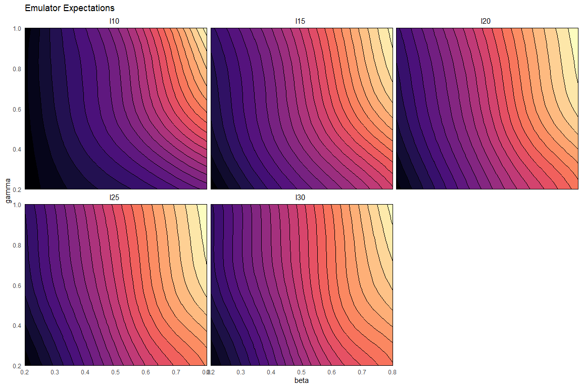

The emulator expectation plots show the structure of the regression surface, which is at most quadratic in its parameters, through a 2D slice of the input space. Here parameters \(\beta\) and \(\gamma\) are selected and we get a plot for each model output. For each pair \((\bar \beta,\bar \gamma)\) the plot shows the expected value produced by the relative emulator at the point \((\bar \beta,\bar \gamma, \delta_{\text{mid-range}}, \mu_{\text{mid-range}})\), where \(\delta_{\text{mid-range}}\) indicates the mid-range value of \(\delta\) and similarly for \(\mu_{\text{mid-range}}\).

To plot the emulators standard deviation we just use emulator_plot passing ‘sd’ as second argument:

emulator_plot(ems0, 'sd', cb=TRUE)

We can see that the emulators reasonably show the structure of the model: the closer the evaluation point is to a training point, the lower the variance (as it ‘knows’ the value at this point). In fact, evaluating these emulators at parameter sets in the training data demonstrates this fact:

em_evals <- ems0$I10$get_exp(train0[,names(ranges)])
all(abs(em_evals - train0$I10) < 10^(-12))
#> [1] TRUE

In the next section we will define the implausibility measure while in section 6 we will explain how to assess whether the emulators we trained are performing as we would expect them to.