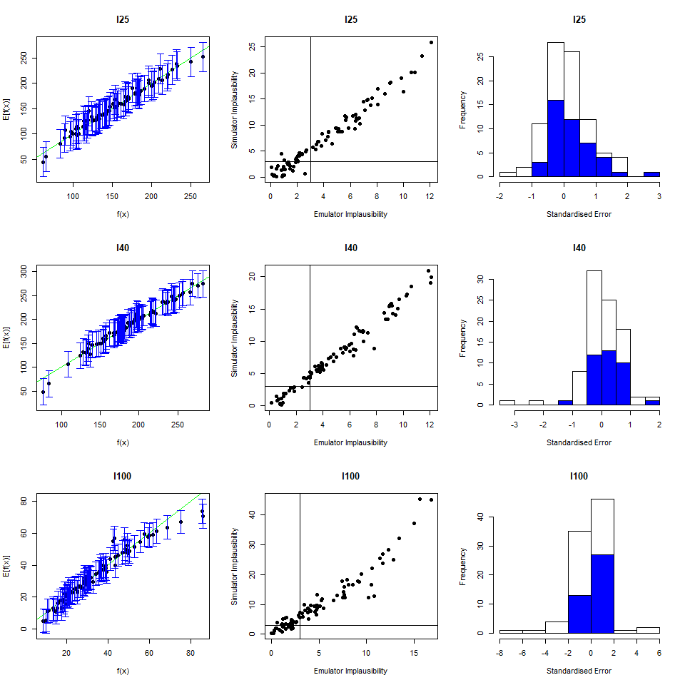
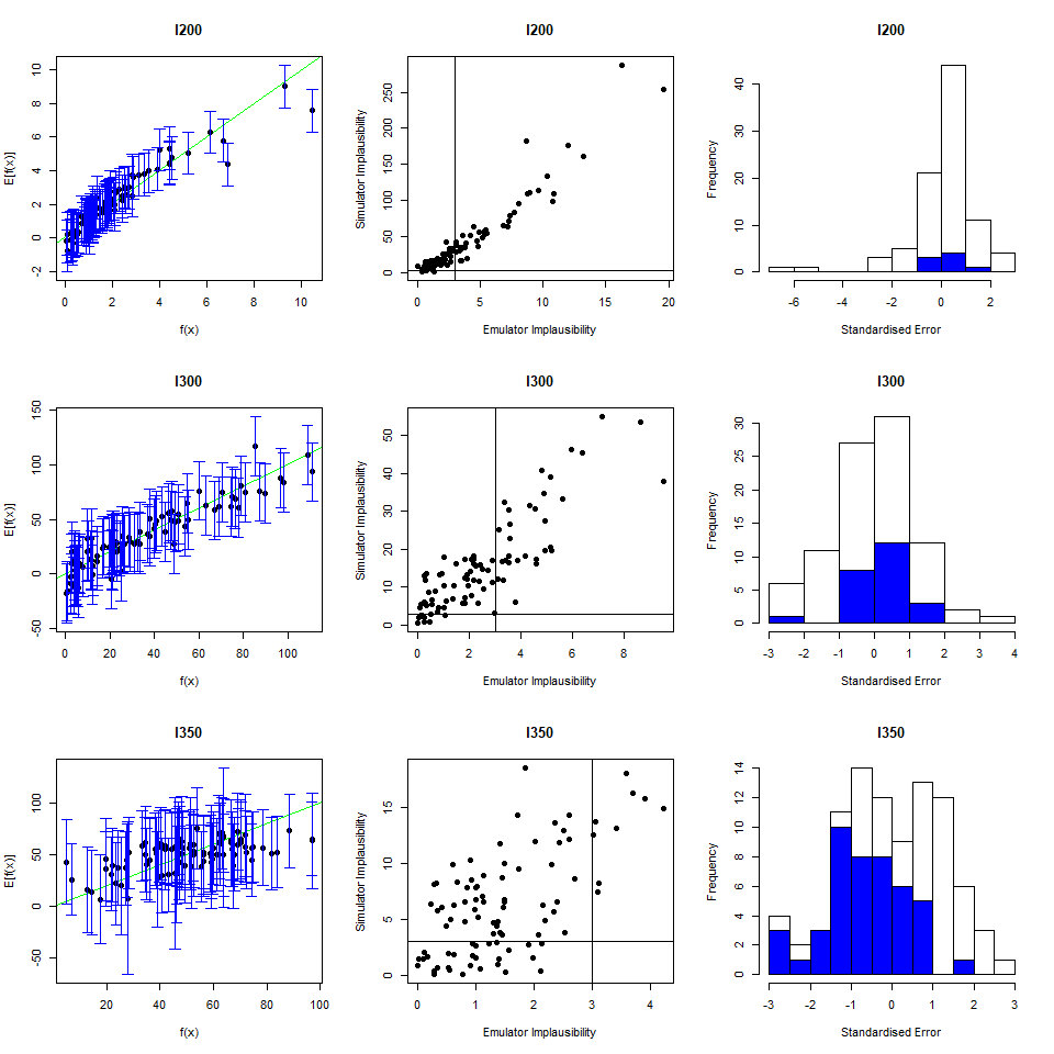
First of all let us take a look at the diagnostics of all the emulators trained in wave 1:
vd <- validation_diagnostics(ems_wave1, validation = validation, targets = targets, plt=TRUE)


Most emulators would benefit from having slightly more conservative emulators, which we can obtain by increasing \(\sigma\). After some trial and error, we chose the following values of sigma for our emulators:
inflations <- c(1.5,1.5,1,1,1,1,1.5,1.5,2,2,1.5,2)
for (i in 1:length(ems_wave1)) {
  ems_wave1[[i]] <- ems_wave1[[i]]$mult_sigma(inflations[[i]])
}
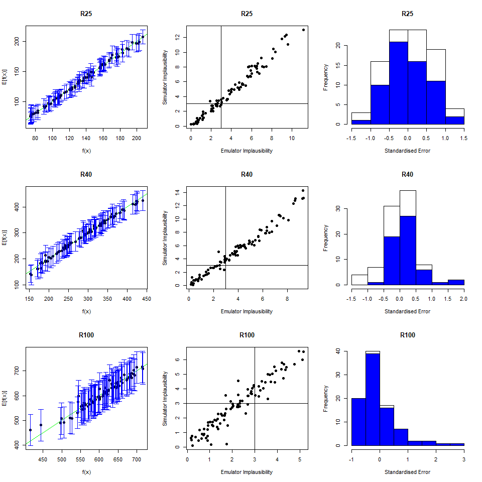
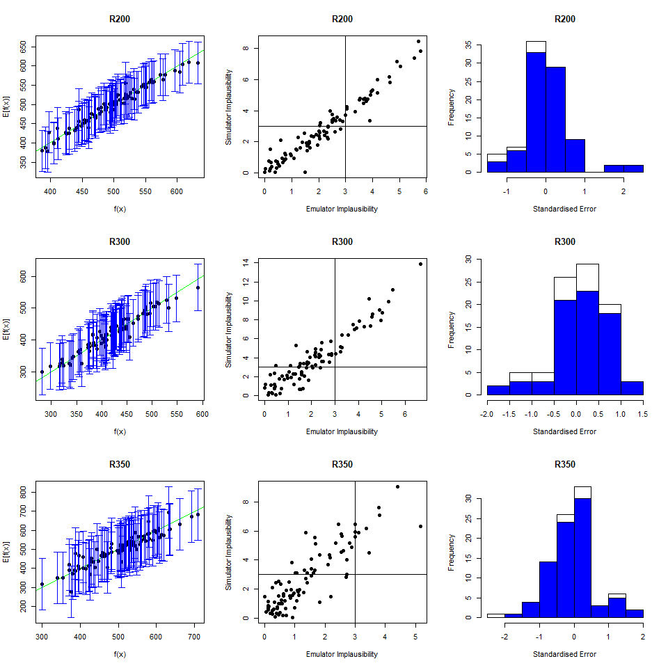
vd <- validation_diagnostics(ems_wave1, validation = validation, targets = targets, plt=TRUE)


The diagnostics look good now. Note that a high increase in sigma, which is sometimes needed to pass diagnostics, may end up producing an emulator that cuts (almost) no space out. This can be checked by looking at the middle diagnostic: if (almost) no validation point has implausiblity above three, then it is advisable not to include the emulator when generating new points. This will avoid adding unnecessary calculations and will not affect the amount of space cut out at that wave. In our specific case, all emulators are contributing to shrinking the space down, so we will include all of them when generating new points:
new_points <- generate_new_design(ems_wave1, 180, targets, verbose = TRUE)
## Proposing from LHS...
## LHS has high yield; no other methods required.
## Selecting final points using maximin criterion...
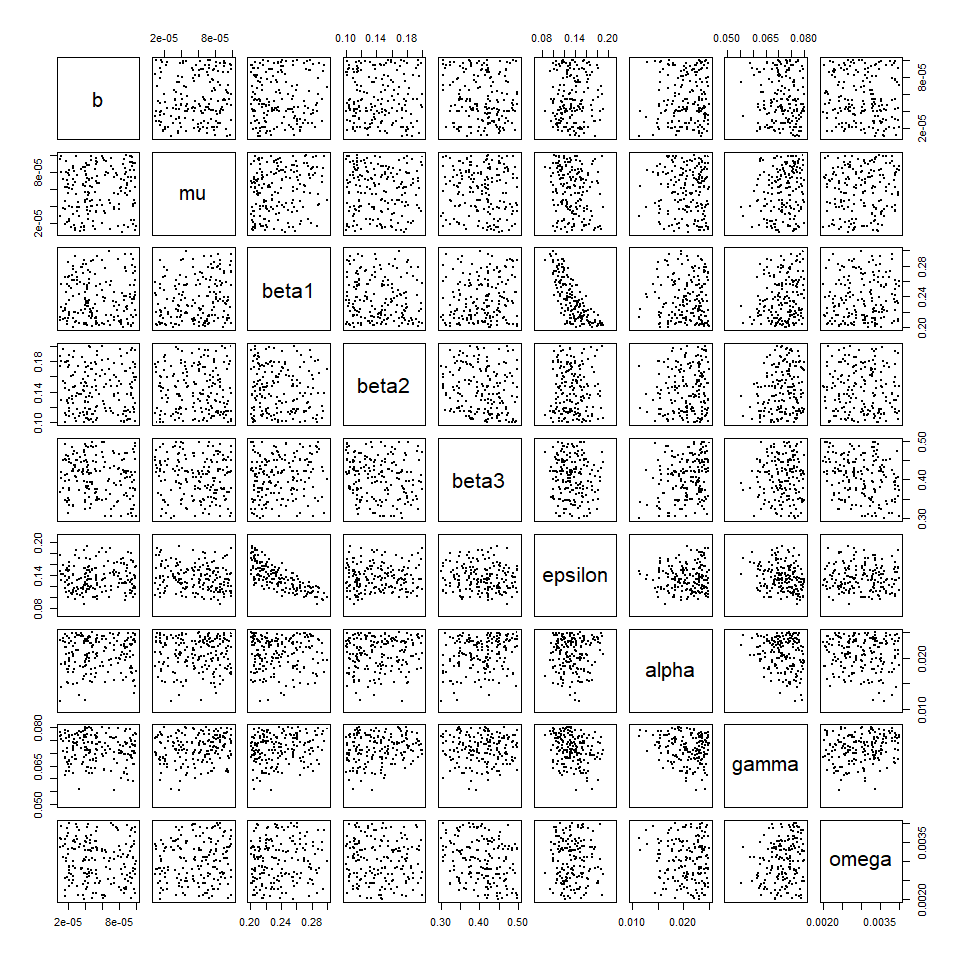
plot_wrap(new_points, ranges)

If we compare the parameter sets we just generated with those generated using non-customised emulators, we note that the space has now been reduced less than before. This happened because our customisation helped us to build more conservative emulators, decreasing the risk of rejecting good parts of the input space. Building emulators carefully ensures that we end up with a set of points that are truly representative of the set of all points that fit the observations (rather than a subset of it).
