4 ‘wave0’ - parameter ranges, targets and design points

A video presentation of this section can be found here.

In this section we set up the emulation task, defining the input parameter ranges, the calibration targets and all the data necessary to build the first wave of emulators.

For the sake of clarity, in this workshop we will adopt the word ‘data’ only when referring to the set of runs of the model that are used to train emulators. Real-world observations, that inform our choice of targets, will instead be referred to as ‘observations.’ Before we tackle the emulation, we need to define some objects. First of all, let us set the parameter ranges:

ranges = list(
  b = c(1e-5, 1e-4), # birth rate
  mu = c(1e-5, 1e-4), # rate of death from other causes
  beta1 = c(0.2, 0.3), # infection rate at time t=0
  beta2 = c(0.1, 0.2), # infection rates at time t=100
  beta3 = c(0.3, 0.5), # infection rates at time t=270
  epsilon = c(0.07, 0.21), # rate of becoming infectious after infection
  alpha = c(0.01, 0.025), # rate of death from the disease
  gamma = c(0.05, 0.08), # recovery rate
  omega = c(0.002, 0.004) # rate at which immunity is lost following recovery
)

We then turn to the targets we will match: the number of infectious individuals \(I\) and the number of recovered individuals \(R\) at times \(t=25, 40, 100, 200, 200, 350\). The targets can be specified by a pair (val, sigma), where ‘val’ represents the measured value of the output and ‘sigma’ represents its standard deviation, or by a pair (min, max), where min represents the lower bound and max the upper bound for the target. Here we will use the former formulation (an example using the latter formulation can be found in Workshop 2):

targets <- list(
  I25 = list(val = 115.88, sigma = 5.79),
  I40 = list(val = 137.84, sigma = 6.89),
  I100 = list(val = 26.34, sigma = 1.317),
  I200 = list(val = 0.68, sigma = 0.034),
  I300 = list(val = 29.55, sigma = 1.48),
  I350 = list(val = 68.89, sigma = 3.44),
  R25 = list(val = 125.12, sigma = 6.26),
  R40 = list(val = 256.80, sigma = 12.84),
  R100 = list(val = 538.99, sigma = 26.95),
  R200 = list(val = 444.23, sigma = 22.21),
  R300 = list(val = 371.08, sigma = 15.85),
  R350 = list(val = 549.42, sigma = 27.47)
)

The ‘sigmas’ in our targets list represent the uncertainty we have about the observations. Note that in general we can also choose to include model uncertainty in the ‘sigmas,’ to reflect how accurate we think our model is. For further discussion regarding model uncertainty, please see Bower, Goldstein, and Vernon (2010), Vernon et al. (2018) or Andrianakis et al. (2015).

Show: More on how targets were set

Since our model is synthetic, we couldn’t rely on observations to define our targets. Instead, we chose the parameter set

chosen_params <- list(b = 1/(76*365), mu = 1/(76*365), beta1 = 0.214, 
                      beta2 = 0.107, beta3 = 0.428, epsilon = 1/7, alpha = 1/50, gamma = 1/14, omega = 1/365)

ran the model with it and used the relevant model outputs as the ‘val’ in targets. The ‘sigma’ components were chosen to be \(5\%\) of the corresponding ‘val.’

Finally we need a set of wave0 data to start. When using your own model, you can create the dataframe ‘wave0’ following the steps below:

• build a named dataframe initial_points containing a space filling set of points, which can be generated using a Latin Hypercube Design or another sampling method of your choice. A rule of thumb is to select at least \(10p\) parameter sets, where \(p\) is the number of parameters in the model. The columns of initial_points should be named exactly as in the list ranges;

• run your model on the parameter sets in initial_points and define a dataframe initial_results in the following way: the nth row of initial_results should contain the model outputs corresponding to the chosen targets for the parameter set in the nth row of initial_points. The columns of initial_results should be named exactly as in the list targets;

• bind initial_points and initial_results by their columns to form the dataframe wave0.

For this workshop, we generate parameter sets using a Latin Hypercube design (see fig. 4.1 for a Latin hypercube example in two dimensions).

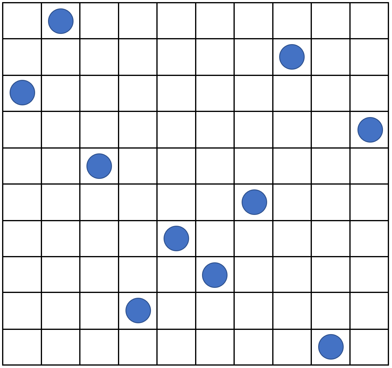
Figure 4.1: An example of Latin hypercube with 10 points in two dimensions: there is only one sample point in each row and each column.

Through the function maximinLHS in the package lhs we create a hypercube design with 90 (10 times the number of parameters) parameter sets for the training set and one with 90 parameter sets for the validation set. After creating the two hypercube designs, we bind them together to create initial_LHS:

initial_LHS_training <- maximinLHS(90, 9)
initial_LHS_validation <- maximinLHS(90, 9)
initial_LHS <- rbind(initial_LHS_training, initial_LHS_validation)

Note that in initial_LHS each parameter is distributed on \([0,1]\). This is not exactly what we need, since each parameter has a different range. We therefore re-scale each component in initial_LHS multiplying it by the difference between the upper and lower bounds of the range of the corresponding parameter and then we add the lower bound for that parameter. In this way we obtain initial_points, which contains parameter values in the correct ranges.

initial_points <- setNames(data.frame(t(apply(initial_LHS, 1, 
                  function(x) x*unlist(lapply(ranges, function(x) x[2]-x[1])) + 
                  unlist(lapply(ranges, function(x) x[1]))))), names(ranges))

We then run the model for the parameter sets in initial_points through the get_results function. This is a helper function that acts as ode_results, but has the additional feature of allowing us to decide which outputs and times should be returned: in our case we need the values of \(I\) and \(R\) at \(t=25, 40, 100, 200, 300, 350\).

initial_results <- setNames(data.frame(t(apply(initial_points, 1, get_results, 
                   c(25, 40, 100, 200, 300, 350), c('I', 'R')))), names(targets))

Finally, we bind the parameter sets initial_points to the model runs initial_results and save everything in the data.frame wave0:

wave0 <- cbind(initial_points, initial_results)

Note that your model can be written in any programming languages and that when using your own model, you can create the ‘wave0’ dataframe however you wish.

References

Andrianakis, Ioannis, Ian R Vernon, Nicky McCreesh, Trevelyan J McKinley, Jeremy E Oakley, Rebecca N Nsubuga, Michael Goldstein, and Richard G White. 2015. “Bayesian History Matching of Complex Infectious Disease Models Using Emulation: A Tutorial and a Case Study on HIV in Uganda.” PLoS Computational Biology 11 (1): e1003968.

Bower, Richard G, Michael Goldstein, and Ian Vernon. 2010. “Galaxy Formation: A Bayesian Uncertainty Analysis.” Bayesian Analysis 5 (4): 619–69.

Vernon, Ian, Junli Liu, Michael Goldstein, James Rowe, Jen Topping, and Keith Lindsey. 2018. “Bayesian Uncertainty Analysis for Complex Systems Biology Models: Emulation, Global Parameter Searches and Evaluation of Gene Functions.” BMC Systems Biology 12 (1): 1–29.