2 The model and calibration setup
In this section we define the model and the calibration setup for our example.
The model that we chose for demonstration purposes is the deterministic SEIRS model used in the deterministic workshop and is described by the following differential equations: \[\begin{align} \frac{dS}{dt} &= b N - \frac{\beta(t)IS}{N} + \omega R -\mu S \\ \frac{dE}{dt} &= \frac{\beta(t)IS}{N} - \epsilon E - \mu E \\ \frac{dI}{dt} &= \epsilon E - \gamma I - (\mu + \alpha) I \\ \frac{dR}{dt} &= \gamma I - \omega R - \mu R \end{align}\] where \(N\) is the total population, varying over time, and the parameters are as follows:
\(b\) is the birth rate,
\(\mu\) is the rate of death from other causes,
\(\beta(t)\) is the infection rate between each infectious and susceptible individual,
\(\epsilon\) is the rate of becoming infectious after infection,
\(\alpha\) is the rate of death from the disease,
\(\gamma\) is the recovery rate and
\(\omega\) is the rate at which immunity is lost following recovery.
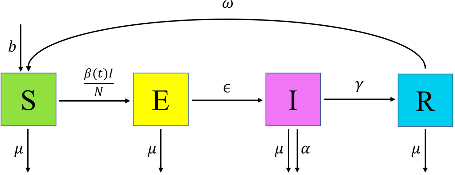
Figure 2.1: SEIRS Diagram
The rate of infection \(\beta(t)\) is set to be a simple linear function interpolating between points, where the points in question are \(\beta(0)=\beta_1\), \(\beta(100) = \beta(180) = \beta_2\), \(\beta(270) = \beta_3\) and where \(\beta_2 < \beta_1 < \beta_3\). This choice was made to represent an infection rate that initially drops due to external (social) measures and then raises when a more infectious variant appears. Here \(t\) is taken to measure days. Below we show a graph of the infection rate over time when \(\beta_1=0.3, \beta_2=0.1\) and \(\beta_3=0.4\):
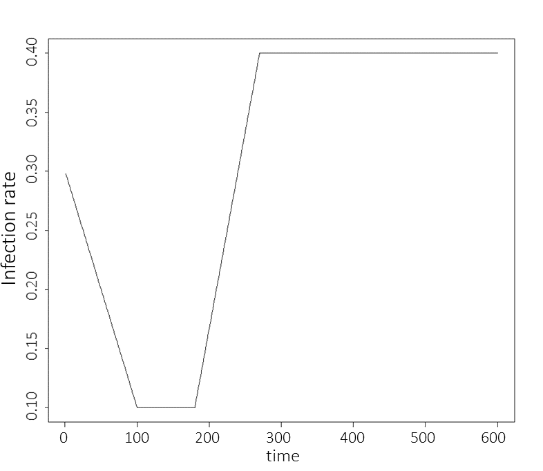
Figure 2.2: Infection rate graph
We now set up the emulation task, defining the input parameter ranges, the calibration targets and all the data necessary to build the first wave of emulators.
First of all, let us set the parameter ranges:
ranges = list(
  b = c(1e-5, 1e-4), # birth rate
  mu = c(1e-5, 1e-4), # rate of death from other causes
  beta1 = c(0.1, 0.5), # infection rate at time t=0
  beta2 = c(0.1, 0.5), # infection rates at time t=100
  beta3 = c(0.1, 0.5), # infection rates at time t=270
  epsilon = c(0.07, 0.21), # rate of becoming infectious after infection
  alpha = c(0.01, 0.025), # rate of death from the disease
  gamma = c(0.05, 0.08), # recovery rate
  omega = c(0.002, 0.004) # rate at which immunity is lost following recovery
)
Note that, even though \(\beta_1\), \(\beta_2\) and \(\beta_3\) have the same initial range \([0.1,0.5]\), when calibrating the model we want to impose \(\beta_2<\beta_1<\beta_3\).
We then turn to the targets we will match: the number of infectious individuals \(I\) and the number of recovered individuals \(R\) at times \(t=25, 40, 100, 200, 200, 350\):
targets <- list(
  I25 = list(val = 115.88, sigma = 5.79),
  I40 = list(val = 137.84, sigma = 6.89),
  I100 = list(val = 26.34, sigma = 1.317),
  I200 = list(val = 0.68, sigma = 0.034),
  I300 = list(val = 29.55, sigma = 1.48),
  I350 = list(val = 68.89, sigma = 3.44),
  R25 = list(val = 125.12, sigma = 6.26),
  R40 = list(val = 256.80, sigma = 12.84),
  R100 = list(val = 538.99, sigma = 26.95),
  R200 = list(val = 444.23, sigma = 22.21),
  R300 = list(val = 371.08, sigma = 15.85),
  R350 = list(val = 549.42, sigma = 27.47)
)
Finally we need an initial design wave0, containing a well-spread set of parameter sets and the corresponding model outputs:
initial_LHS_training <- maximinLHS(90, 9)
initial_LHS_validation <- maximinLHS(90, 9)
initial_LHS <- rbind(initial_LHS_training, initial_LHS_validation)
initial_points <- setNames(data.frame(t(apply(initial_LHS, 1,
                  function(x) x*unlist(lapply(ranges, function(x) x[2]-x[1])) +
                  unlist(lapply(ranges, function(x) x[1]))))), names(ranges))
initial_results <- setNames(data.frame(t(apply(initial_points, 1, get_results,
                   c(25, 40, 100, 200, 300, 350), c('I', 'R')))), names(targets))
wave0 <- cbind(initial_points, initial_results)