3 Constructing the emulators

The first task that the full_wave function accomplishes, is to build the emulators based on the training data. We start this section by establishing the structure of the emulators that we want to construct. We then show how to build emulators step by step.

3.1 Background: the structure of an emulator

An emulator is a way of representing our beliefs about the behaviour of an unknown function. In our example we have a stochastic model and we choose the unknown function to be the mean of each of the model outputs over multiple runs. Given a set of model runs, we can use the emulator to get expectation and variance for a model output at any parameter set, without the need to run the model at the chosen set. Note that more sophisticated approaches are possible when working with stochastic models: apart from the mean of outputs, other features, such as the variance or various quantiles can be approximated through emulators.

In this tutorial, we will construct an emulator for each of the model outputs separately (even though more complex techniques that combine outputs are available). The general structure of a univariate emulator is as follows: \[f(x) = g(x)^T \beta + u(x),\] where \(g(x)\) is a vector of known deterministic regression functions, \(\beta\) is a vector of regression coefficients, and \(u(x)\) is a Gaussian process with zero mean. In our tutorial the correlation of the process \(u(x)\) is assumed to be in the following form, for two parameter sets \(x\) and \(x^{\prime}\): \[\sigma^2 \left[(1-\delta) c(x,x^{\prime}) + \delta I_{\{x=x^\prime\}}\right].\] Here \(\sigma^2\) is the (prior) emulator variance and \(c(x,x^{\prime})\) is a correlation function; the simplest such function is squared-exponential \[c(x,x^{\prime}) = \exp\left(-\sum\limits_{i}\frac{(x_{i}-x_{i}^{\prime})^2}{\theta_i^2}\right).\] The ‘nugget’ term \(\delta I_{\{x=x^{\prime}\}}\) operates on all the parameters in the input space and also represents the proportion of the overall variance due to the ensemble variability. This term also ensures that the covariance matrix of \(u(x)\) is not ill-conditioned, making the computation of its inverse possible (a key operation in the training of emulators, see Appendix A). The \(\theta_i\) hyperparameters are the correlation lengths for the emulator. The size of the correlation lengths determine how close two parameter sets must be in order for the corresponding residual values to be highly correlated. A smaller \(\theta_i\) value means that we believe that the function is less smooth with respect to parameter \(i\), and thus that the values for the corresponding parameters \(x_i\) and \(x_i^{\prime}\) must be closer together in order to be highly correlated. The simplifying assumption that all the correlation length parameters are the same, that is \(\theta_i = \theta\) for all \(i\), can be made, but more sophisticated versions are of course available. In such case, the larger \(\theta\) is, the smoother the local variations of the emulators will be.

Show: Dealing with high dimensions

Since in this tutorial we are working with a low-dimensional input space, we chose a relatively basic structure for our emulator. Note that more complex structures may be needed when dealing with higher dimensional problems, since the complexity of the emulation process increases significantly with dimensionality. There are several ways of tackling high dimensional problems. One of these consists in reducing the number of dimensions by selecting the variables that explain the data the most. More info on active variables can be found in Appendix B.

We would like to warn the reader that several emulator structures and correlation functions are available. Alternatives choices to the ones made above are discussed in Appendix B.

3.2 Constructing the emulators step by step

To construct the emulators, two steps are required:

1. We create a set of ‘initial’ emulators ems0 by fitting a regression surface to train0. These simple emulators will provide us with estimates for the regression surface parameters and the basic correlation specifications;

2. The emulators ems0 constitute our prior which we adjust to the training data through the Bayes Linear update formulae. In this way we obtain the final version of our first wave emulators: ems0_adjusted.

Let us now go through each step in detail.

3.2.1 Step 1

The function emulator_from_data creates the initial emulators for us. We pass emulator_from_data the training data, the name of the model outputs we want to emulate, the list of parameter ranges and the ensemble variability. Taken this information, emulator_from_data finds both the regression parameters and the active parameters for each of the indicated model outputs. Model selection is performed through stepwise addition or deletion (as appropriate), using the AIC criterion to find the minimal best fit. Note that the default behaviour of emulator_from_data is to fit a quadratic regression surface. If we want instead a linear regression surface, we just need to set quadratic=FALSE. We note that in principle we can insert basis functions of any form for the regression surface.

evs <- apply(wave0[10:ncol(wave0)], 2, mean)
ems0 <- emulator_from_data(train0, output_names, ranges, ev=evs, lik.method = 'my')
ems0[[1]]
#> Parameters and ranges:  beta: c(0.2, 0.8); gamma: c(0.2, 1); delta: c(0.1, 0.5); mu: c(0.1, 0.5) 
#> Specifications: 
#>   Basis Functions:  (Intercept); beta; gamma; delta; beta:gamma; beta:delta; gamma:delta 
#>   Active variables:  beta; gamma; delta 
#>   Beta Expectation:  100.14; 94.8268; 39.3626; -104.0459; 40.5446; -71.8908; -31.4994 
#>   Beta Variance (eigenvalues):  0; 0; 0; 0; 0; 0; 0 
#> Correlation Structure: 
#>   Variance:  651.438 
#>   Expectation:  0 
#>   Correlation length:  1.241873 
#>   Nugget term:  0.1522625 
#> Mixed covariance:  0 0 0 0 0 0 0

Note that we calculated the ensemble variability evs taking the mean of the column \(EV\) in wave0. The function emulator_from_data uses evs to estimate the delta parameter, i.e. the proportion of the overall variance due to the ensemble variability.

Show: More details about the ems0 objects

The print statement provides an overview of the emulator specifications and correlation structure, including

• Basis Functions: here we have the four parameters beta, gamma, delta, mu and some products of them, since we chose quadratic regression. Note that beta:mu and all pure quadratic terms (such as beta:beta) are not listed: this means that stepwise addition and deletion led to discarding them,

• Active variables,

• first and second order specifications for \(\beta\) and \(u(x)\). Note that by default emulator_from_data assumes that \(\text{Var}[\beta]=0\): the regression surface is known and coefficients are fixed. This explains why Beta Variance and Mixed Covariance (which shows the covariance of \(\beta\) and \(u(x)\)) are both zero. One can set beta.var=TRUE in order to consider the beta parameters as random variables.

We can plot the emulators to see how they represent the output space: the emulator_plot function does this for emulator expectation, variance, standard deviation, and implausibility (more on which later). Note that all functions in the emulatorr package that produce plots have a colorblind-friendly option: it is sufficient to specify cb=TRUE.

for (i in 1:length(ems0)) ems0[[i]]$output_name <- output_names[i]
names(ems0) <- output_names
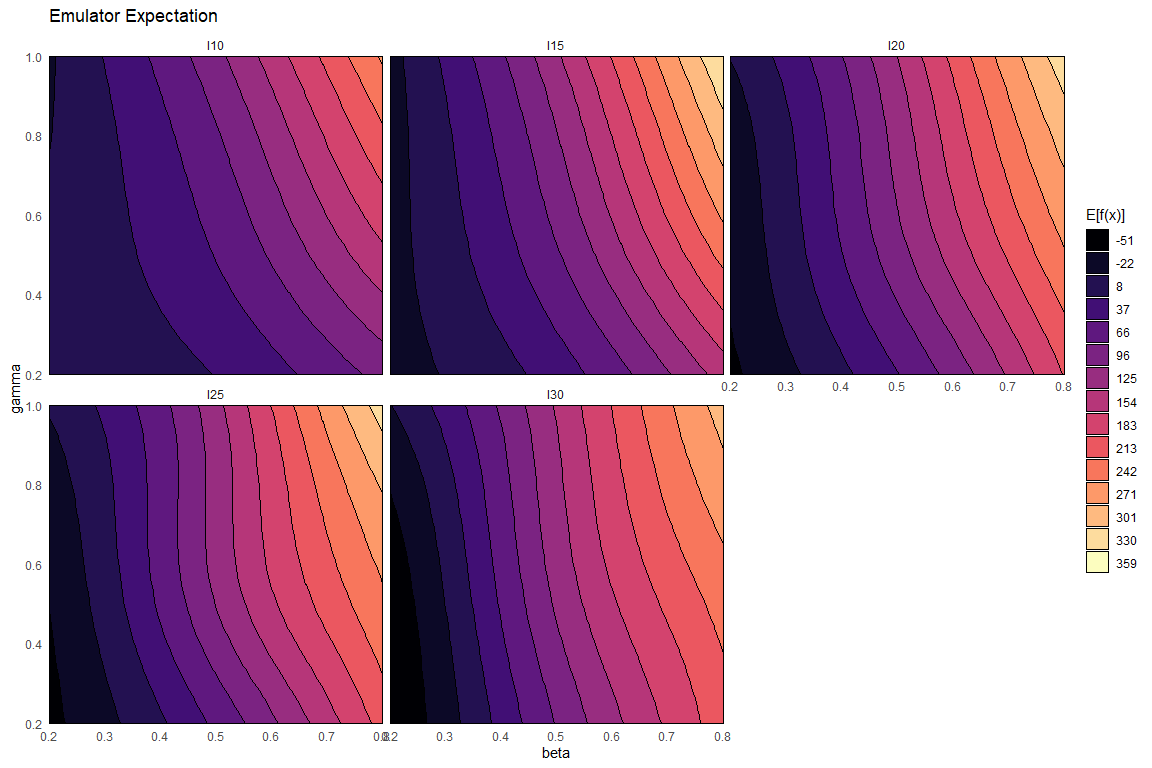
emulator_plot(ems0)

The emulator expectation plots show the structure of the regression surface, which is at most quadratic in its parameters, through a 2D slice of the input space. Here parameters \(\beta\) and \(\gamma\) are selected and we get a plot for each model output. For each pair \((\bar \beta,\bar \gamma)\) the plot shows the expected value produced by the relative emulator at the point \((\bar \beta,\bar \gamma, \delta_{\text{mid-range}}, \mu_{\text{mid-range}})\), where \(\delta_{\text{mid-range}}\) indicates the mid-range value of \(\delta\) and similarly for \(\mu_{\text{mid-range}}\).

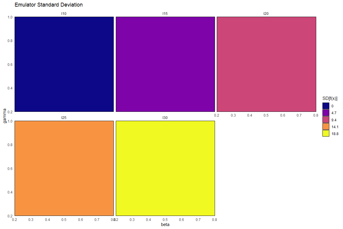
To plot the emulators standard deviation we just use emulator_plot passing ‘sd’ as second argument:

emulator_plot(ems0, 'sd')

Here we immediately see that the emulator variance (or equivalently, standard deviation) is simply constant across the parameter space for each emulated output. This is not what we want though, since one would expect emulators to be less uncertain around the parameter sets that have been evaluated by the computer model. This will be taken care of in the next step.

3.2.2 Step 2

We now use the adjust method on our emulators to obtain the final Bayes Linear version of our wave0 emulators:

ems0_adjusted <- map(seq_along(ems0), ~ems0[[.]]$adjust(train0, output_names[[.]]))

Note that the adjust method works with the data in train0 exactly as the function emulator_from_data did: it performs Bayes Linear adjustment, given the data. This function creates a new emulator object with the adjusted expectation and variance of beta as the primitive specifications, and supplies the values for the new emulator to compute the adjusted expectation and variance of \(u(x)\), and the adjusted \(Cov[\beta, u(x)]\). Due to the update formulae, the correlation structure now depends on where in the input space it is evaluated.

names(ems0_adjusted) <- output_names
emulator_plot(ems0_adjusted)

emulator_plot(ems0_adjusted, params = c('gamma', 'delta'), var = 'sd')

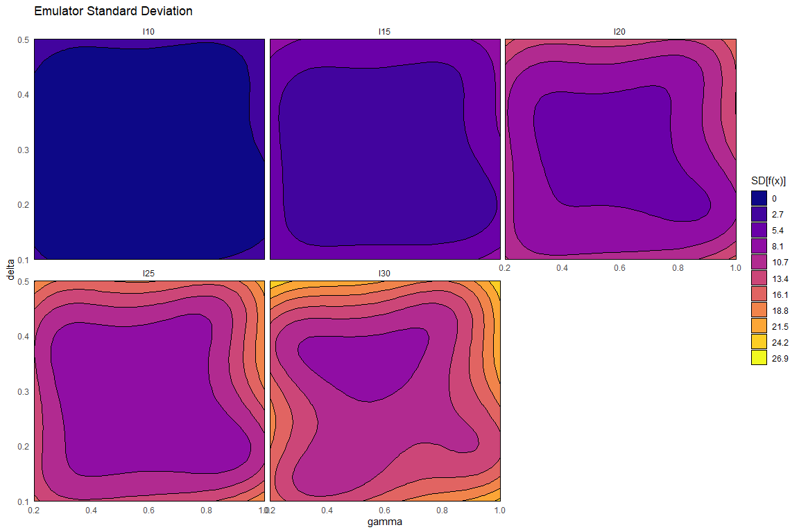
We can see that the adjusted emulators more reasonably show the structure of the model. The variance has been updated: the closer the evaluation point is to a training point, the lower the variance (as it ‘knows’ the value at this point). In fact, evaluating these emulators at parameter sets in the training data demonstrates this fact:

em_evals <- ems0_adjusted$I10$get_exp(train0[,names(ranges)])
all(abs(em_evals - train0$I10) < 10^(-12))
#> [1] TRUE

In the next section we will define the implausibility measure while in section 5 we will explain how to assess whether the emulators we trained are performing as we would expect them to.