11 Dealing with bimodality

A video presentation of this section can be found here.

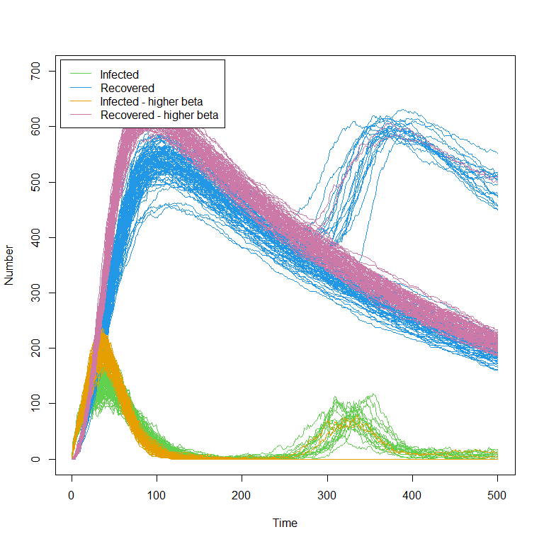
In the previous sections of this workshop we dealt with stochasticity, but not with bimodality, i.e. when one can perform multiple repetitions at a given parameter set and find two distinct classes of behaviour. This is because our SEIRS model did not show any bimodal behaviour in the outputs for the times considered, i.e. for \(t\) up to \(200\). Let us suppose now that we are interested also in later times. Running the model on chosen_params using get_results up to time \(t=500\) and plotting the results for “I” and “R” we obtain:

solution <- get_results(chosen_params, outs = c("I", "R"), 
                        times = c(25, 40, 100, 200, 300, 400, 500), raw = TRUE)
plot(0:500, ylim=c(0,700), ty="n", xlab = "Time", ylab = "Number")
for(j in 3:4) for(i in 1:100) lines(0:500, solution[,j,i], col=(3:4)[j-2], lwd=0.3)
legend('topleft', legend = c('Infected', "Recovered"), lty = 1, 
       col = c(3,4), inset = c(0.05, 0.05))

The most common example of bimodality, ‘take off vs die out,’ now enters the picture: from time \(t=250\) on, there are a large number of trajectories in green that have zero infected individuals (note the horizontal green line) and a few trajectories where transmission takes off again, producing a second wave of the epidemic (around \(t=300\)).

Task

Investigate how different parameter sets give rise to different levels of bimodality.

Show: R tip

Copy the code below, modify the value of (some) parameters and run it.

example_params <- c(
  b = 1/(76*365),  # birth rate
  mu = 1/(76*365),  # rate of death from other causes
  beta1 = 0.214, beta2 = 0.107, beta3 = 0.428,  # infection rate between each infectious and susceptible individual
  epsilon = 1/7,  # rate of becoming infectious after infection
  alpha = 1/50,  # rate of death from the disease
  gamma = 1/14,  # recovery rate
  omega = 1/365  # rate at which immunity is lost following recovery
)
solution <- get_results(example_params, outs = c("I", "R"), 
                        times = c(25, 40, 100, 200), raw = TRUE)
plot(0:200, ylim=c(0,700), ty="n", xlab = "Time", ylab = "Number")
for(j in 3:4) for(i in 1:100) lines(0:200, solution[,j,i], col=(3:4)[j-2], lwd=0.3)
legend('topleft', legend = c('Infected', "Recovered"), lty = 1, 
       col = c(3,4), inset = c(0.05, 0.05))

Solution

Let us see what happens when we simulate a higher rate of infection between each infectious and susceptible:

higher_beta_params <- c(
  b = 1/(76*365),
  mu = 1/(76*365),
  beta1 = 0.3, beta2 = 0.1, beta3 = 0.5,
  sigma = 1/7,
  alpha = 1/50,
  gamma = 1/14,
  omega = 1/365
)
higher_beta_solution <- get_results(higher_beta_params, outs = c("I", "R"), 
                        times = c(25, 40, 100, 200, 300, 400, 500), raw = TRUE)
plot(0:500, ylim=c(0,700), ty="n", xlab = "Time", ylab = "Number")
for(j in 3:4) for(i in 1:100) lines(0:500, solution[,j,i], col=(3:4)[j-2], lwd=0.3)
for(j in 3:4) for(i in 1:100) lines(0:500, higher_beta_solution[,j,i], 
                                    col=(c("#E69F00","#CC79A7"))[j-2], lwd=0.3)
legend('topleft', legend = c('Infected', "Recovered", "Infected - higher beta", 
                             "Recovered - higher beta"), lty = 1, 
       col = c(3,4,"#E69F00","#CC79A7"), inset = c(0.01, 0.01))

We see that the peaks of recovered and infectious individuals during the first wave have now increased, as expected. Also note how increasing the transmission rate reduced the role of bimodality (very few trajectories in orange take off after the first wave): the fact that more individuals get now infected during the first wave (around \(t=50\)), makes the chances of a second “wave” around time \(t=300\) lower.

In the following subsections we will describe how to deal with bimodality when performing history matching with emulation. Since most parts of the process are very similar to what we have seen already for stochastic models, we will only discuss the areas where the process changes.

Similar to the philosophy of the previous sections, we will match the observed data to the mean within each of the two modes. This can be used to then exclude a large portion of the input space without resorting to modelling the specific distributional form of the model output. In later workshops we will also learn to match to the set of possible realisations of a stochastic model, by emulating its covariance structure.

11.1 ‘bimodal_wave0’ - design points

While the parameters’ ranges are the same as before, we need to redefine the targets’ list, adding values for times later than \(t=200\):

bimodal_targets <- list(
  I25 = list(val = 115.88, sigma = 5.79),
  I40 = list(val = 137.84, sigma = 6.89),
  I100 = list(val = 26.34, sigma = 1.317),
  I200 = list(val = 0.68, sigma = 0.034),
  I250 = list(val = 9.67, sigma = 4.76),
  I400 = list(val = 15.67, sigma = 5.36),
  I500 = list(val = 14.45, sigma = 5.32),
  R25 = list(val = 125.12, sigma = 6.26),
  R40 = list(val = 256.80, sigma = 12.84),
  R100 = list(val = 538.99, sigma = 26.95),
  R200 = list(val = 444.23, sigma = 22.21),
  R250 = list(val = 361.08, sigma = 25.85),
  R400 = list(val = 569.39, sigma = 26.52),
  R500 = list(val = 508.64, sigma = 28.34)
)

Note that these are the same exact targets chosen for the deterministic workshop, Workshop 1.

Since we are now interested in times after \(t=200\) too, we need to rerun the parameter sets in initial_points, obtaining bimodal_initial_results. We then bind all elements in bimodal_initial_results to obtain a dataframe bimodal_wave0, which we split into a training and a validation set:

bimodal_initial_results <- list()
with_progress({
  p <- progressor(nrow(initial_points))
for (i in 1:nrow(initial_points)) {
  model_out <- get_results(unlist(initial_points[i,]), nreps = 50, outs = c("I", "R"), 
                           times = c(25, 40, 100, 200, 250, 400, 500))
  bimodal_initial_results[[i]] <- model_out
  p(message = sprintf("Run %g", i))
}
})
bimodal_wave0 <- data.frame(do.call('rbind', bimodal_initial_results))
bimodal_all_training <- bimodal_wave0[1:5000,]
bimodal_all_valid <- bimodal_wave0[5001:7500,]
bimodal_output_names <- c("I25", "I40", "I100", "I200", "I250", "I400", "I500", 
                          "R25", "R40", "R100", "R200", "R250", "R400", "R500")

11.2 Bimodal Emulators

To train bimodal emulators we use the function emulator_from_data specifying emulator_type = 'multistate', which requires the training data, the names of the outputs to emulate, and the ranges of the parameters:

bimodal_emulators <- emulator_from_data(bimodal_all_training, 
                                        bimodal_output_names, ranges,
                                        emulator_type = 'multistate')

Behind the scenes, this function does the following:

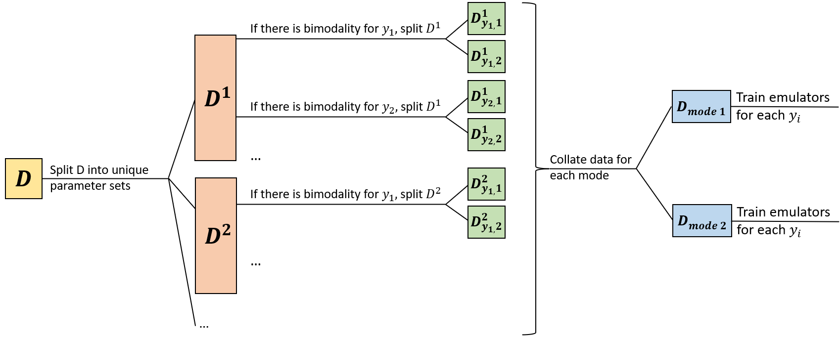
• First it looks at the provided training data and identifies which of the outputs are bimodal (see box below if interested in the method used to identify bimodal outputs).

• For the outputs where bimodality is found, the repetitions at each parameter set are clustered into two subsets, based on the mode they belong to.

• For outputs without bimodality, stochastic emulators are trained as before. For outputs with bimodality, variance and mean emulators are trained separately for each of the two modes. To access the mean emulators for the first mode, we type bimodal_emulators$mode1$expectation, and to access the variance emulators for the second mode we type bimodal_emulators$mode2$variance.

• Finally, an emulator for the proportion of points in each mode is also trained (this is a single emulator, as in the deterministic case). This emulator can be accessed by typing bimodal_emulators$prop and will be referred to as proportion emulator.

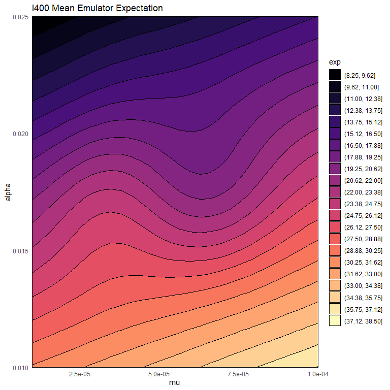
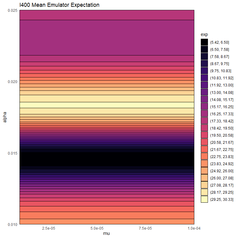
Let us now plot the expectation of the mean emulator of \(R400\) for each mode fixing all non-shown parameters to their values in chosen_params:

emulator_plot(bimodal_emulators$mode1$expectation$R400, params = c('mu', 'alpha'), 
              fixed_vals = chosen_params[!names(chosen_params) %in% c('mu', 'alpha')])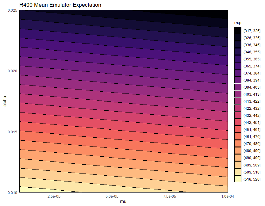

emulator_plot(bimodal_emulators$mode2$expectation$R400, params = c('mu', 'alpha'), 
              fixed_vals = chosen_params[!names(chosen_params) %in% c('mu', 'alpha')])

We notice that mode 2 tends to contain higher values than mode 1. This indicates that mode 1 is the one where the infection dies out.

It is also instructive to plot the expectation of the proportion emulator. We use the argument fixed_vals to set the parameters that are not shown in the plot to be as in chosen_params:

emulator_plot(bimodal_emulators$prop, params = c('alpha', 'epsilon'), 
              fixed_vals = chosen_params[!names(chosen_params) %in% c('alpha' ,'epsilon')]) +
              geom_point(aes(x=1/7, y=1/50), size=3)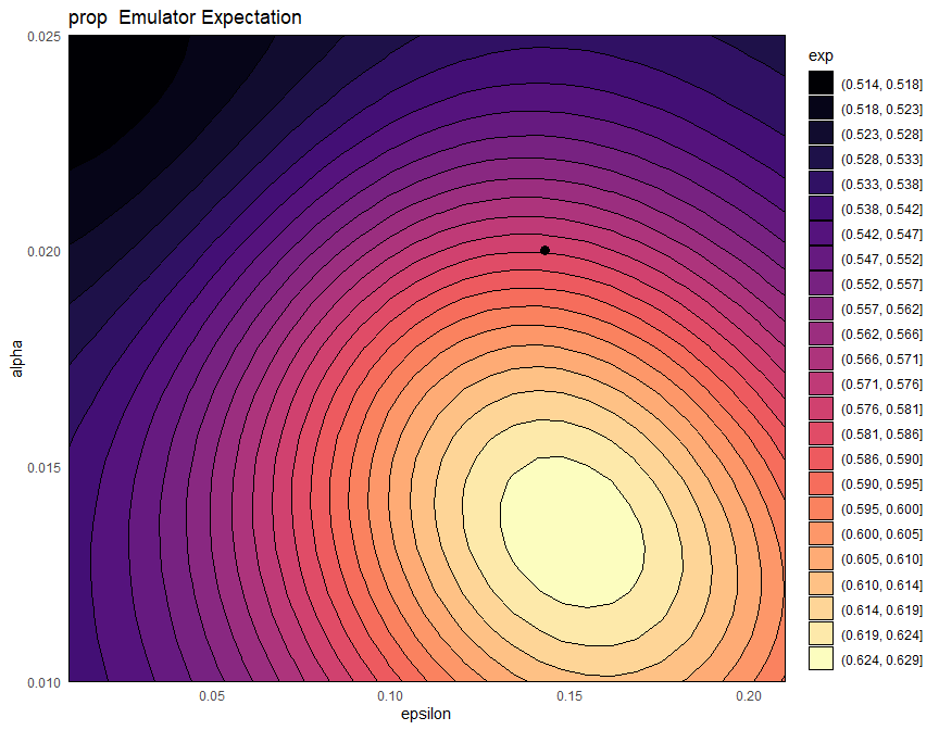

The plot shows that the proportion of points in mode 1, where the infection dies out, is around 0.58. This is in accordance with the plot produced at the beginning of this section, where the infection died out on the majority of trajectories.

Show: How are bimodal outputs identified?

Suppose we are given a dataframe containing parameter sets (with repetitions) and the corresponding outputs. An individual row of that dataframe would be of the form \((x, y) = (x_1, x_2, x_3, …, x_p, y_1, y_2, … y_n)\) where \(x\) are the paramters and \(y\) the outputs. To check and classify bimodality we follow the steps below:

1. We split the dataframe into unique parameter sets, collecting repetitions for each parameter set together. For each unique parameter set \(\bar{x}\) and each \(i=1,...,n\), we use clustering on \(y_i\) (with finite normal mixture models), allowing a maximum of two clusters. If the optimal clustering has two clusters, we consider the output \(y_i\) to be bimodal at \(\bar{x}\); otherwise we consider it unimodal.

2. If for all parameter sets and all outputs, the optimal clustering is a single cluster, then we have no bimodality: we then perform stochastic emulation using emulator_from_data with emulator_type = 'variance'. Otherwise, for each output \(y_i\) and each unique parameter set \(\bar{x}\):

   2.1. If there is no bimodality in \(y_i\) for \(\bar{x}\), then all the data from \(\bar{x}\) for \(y_i\) will be used in each mode.

   2.2. If there is bimodality in \(y_i\) for \(\bar{x}\), then we determine which of the repetitions in the parameter set \(\bar{x}\) correspond to the identified bimodality (again, using clustering). The dataset for that parameter set \(\bar{x}\) gets split into two: one for each mode.

3. We collate the data for each mode, resulting in (for each output) two dataframes of repetitions. Note that it is unlikely that each mode gets the same number of repetitions to train to.

4. For each mode, we train a list of emulators (one for each output) using the data appropriate to that mode. Note that there is a slight redundancy here, in that if there was no bimodality in an output for any parameter choices, then we have essentially trained the same emulator twice.

The process described above is schematically represented in the figure below:

Task

Confirm that mode 1 is where the infection dies out by comparing the plots of the expectation of the mean emulator for \(I400\) for both modes.

Solution

We use emulator_plot to produce the suggested plots:

emulator_plot(bimodal_emulators$mode1$expectation$I400, params = c('mu', 'alpha'))

emulator_plot(bimodal_emulators$mode2$expectation$I400, params = c('mu', 'alpha'))

The values in the plot for mode 1 are lower than those for mode 2: this reflects the fact that mode 2 experiences a second wave around \(t=300\), while in mode 1 the infection dies out after the first wave (around \(t=40\)).

11.3 Implausibility

Since we are now in a bimodal setting, we want to regard a point as non-implausible for a given target if it is valid with respect to either mode. This is the default behaviour of the package, when dealing with bimodal emulators.

For a given output and a given point, the implausibility for mode 1 and the implausibility for mode 2 are calculated, and the minimum of them is taken. The maximum (or second-maximum, third-maximum etc) of this collection of minimised implausibilities is then selected, depending on the user choice. For example, to plot the maximum of these minimised implausibilities, we set plot_type to nimp:

emulator_plot(bimodal_emulators, plot_type = 'nimp', targets = bimodal_targets, 
              params = c('alpha', 'epsilon'))

Task

Set the argument plot_type to imp to produce implausibility plots for each output, for mode 1 and mode 2. Which implausibility plots are the same for each mode, and which are different? Why?

Solution

Setting plot_type='imp' in emulator_plot and passing it either subset_emulators(bimodal_emulators, output_names[-c(7,14)])$mode1 or subset_emulators(bimodal_emulators, output_names[-c(7,14)])$mode2, we get:

emulator_plot(bimodal_emulators$mode1, plot_type = 'imp', 
              targets = bimodal_targets, params = c('omega', 'epsilon'))

emulator_plot(bimodal_emulators$mode2, plot_type = 'imp', 
              targets = bimodal_targets, params = c('omega', 'epsilon'))

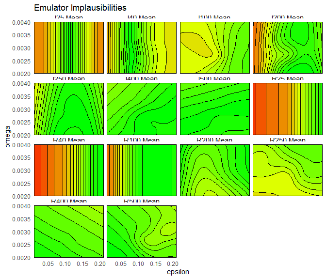
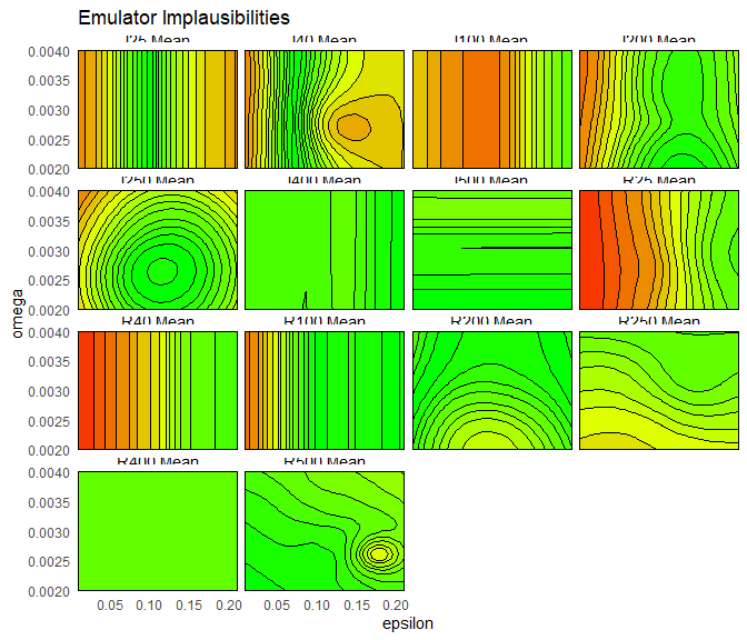The implausibility plots are the same between modes for early times (\(t=25,40,100\)) and different between modes for later outputs. This makes sense, since bimodality, which enters the picture after the first wave, does not play a role in earlier times.

11.4 Emulator diagnostics

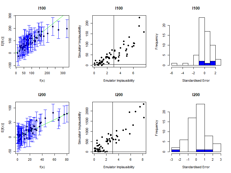
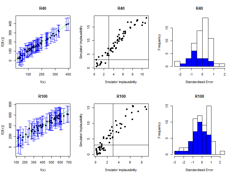
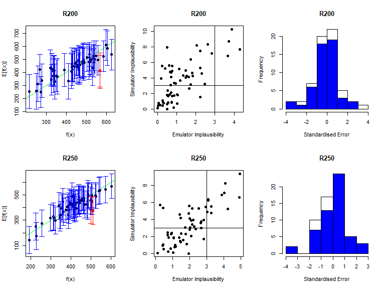
As before, the function validation_diagnostics can be used to get three diagnostics for each emulated output. For example, to produce diagnostics for the first four emulators we type:

vd <- validation_diagnostics(bimodal_emulators, bimodal_targets, bimodal_all_valid, 
                             plt=TRUE, row=2)

## Warning in fanny(suppressWarnings(daisy(v_outputs)), k = 2): the memberships are
## all very close to 1/k. Maybe decrease 'memb.exp' ?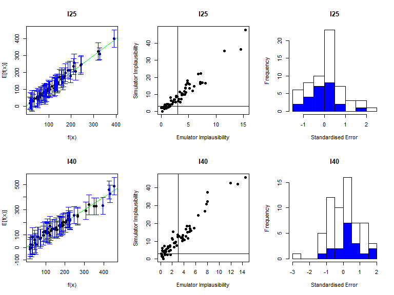

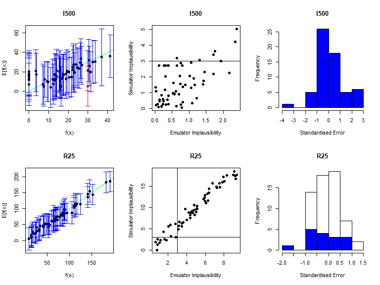
You may have noticed that in the first column we have more points plotted than we have validation points. This is because we do diagnostics for each mode for each output, i.e. we compare the predictions of the mean emulators for mode 1 and mode 2 with the model output values, which are also clustered in two subsets, due to bimodality.

As in the deterministic case, one can enlarge the \(\sigma\) values to obtain more conservative emulators, if needed. For example, to double the \(\sigma\) value for the mean emulators for \(I500\) in both modes we would type:

bimodal_emulators$mode1$expectation$I500 <- bimodal_emulators$mode1$expectation$I500$mult_sigma(2)
bimodal_emulators$mode2$expectation$I500 <- bimodal_emulators$mode2$expectation$I500$mult_sigma(2)

11.5 Proposing new points

Generating a set of non-implausible points, based on the trained emulators, is done in exactly the same way as it was in Section 8, using the function generate_new_design. In this case we need to use the function subset_emulators to remove the emulators for the outputs at \(t=450\) (the seventh and fourteenth emulators), for which we did not set targets:

new_points <- generate_new_design(bimodal_emulators, 150, bimodal_targets, nth=1)

Similarly, performing the second wave is done in the same as it was in Section 9, replacing emulator_type = 'variance' with emulator_type = 'multistate' when calling emulator_from_data.