7 Emulator diagnostics

A video presentation of this section can be found here.

The function validation_diagnostics can be used as in the deterministic case, to get three diagnostics for each emulated output.

Show: Remind me of what each diagnostics means

The first column shows the emulator outputs plotted against the model outputs. In particular, the emulator expectation is plotted against the model output for each validation point, providing the dots in the graph. The emulator uncertainty at each validation point is shown in the form of a vertical interval that goes from $3\sigma$ below to $3\sigma$ above the emulator expectation, where $\sigma$ is the emulator variance at the considered point. An ‘ideal’ emulator would exactly reproduce the model results: this behaviour is represented by the green line $f(x)=E[f(x)]$ (this is a diagonal line, visible here only in the bottom left and top right corners). Any parameter set whose emulator prediction lies more than $3\sigma$ away from the model output is highlighted in red. Note that we do not need to have no red points for the test to be passed: since we are plotting $3\sigma$ bounds, statistically speaking it is ok to have up to $5\%$ of validation points in red (see Pukelsheim’s $3\sigma$ rule).

The second column compares the emulator implausibility to the equivalent model implausibility (i.e. the implausibility calculated replacing the emulator output with the model output). There are three cases to consider:

The emulator and model both classify a set as implausible or non-implausible (bottom-left and top-right quadrants). This is fine. Both are giving the same classification for the parameter set.
The emulator classifies a set as non-implausible, while the model rules it out (top-left quadrant): this is also fine. The emulator should not be expected to shrink the parameter space as much as the model does, at least not on a single wave. Parameter sets classified in this way will survive this wave, but may be removed on subsequent waves as the emulators grow more accurate on a reduced parameter space.
The emulator rules out a set, but the model does not (bottom-right quadrant): these are the problem sets, suggesting that the emulator is ruling out parts of the parameter space that it should not be ruling out. As for the first test, we should be alarmed only if we spot a systematic problem, with $5\%$ or more of the points in the bottom-right quadrant.

Finally, the third column gives the standardised errors of the emulator outputs in light of the model output: for each validation point, the difference between the emulator output and the model output is calculated, and then divided by the standard deviation $\sigma$ of the emulator at the point. The general rule is that we want our standardised errors to be somewhat normally distributed around $0$, with $95\%$ of the probability mass between $-3$ and $3$. The blue bars indicate the distribution of the standardised errors when we restrict our attention only to parameter sets that produce outputs close to the targets. When looking at the standard errors plot, we should ask ourselves at least the following questions:

Is more than $5\%$ of the probability mass outside the interval $[-3,3]$? If the answer is yes, this means that, even factoring in all the uncertainties in the emulator and in the observed data, the emulator output is too often far from the model output.
Is $95\%$ of the probability mass concentrated in a considerably smaller interval than $[-3,3]$ (say, for example, $[-0.5,0.5]$)? For this to happen, the emulator uncertainty must be quite large. In such case the emulator, being extremely cautious, will cut out a small part of the parameter space and we will end up needing many more waves of history matching than are necessary.
Is the histogram skewing significantly in one direction or the other? If this is the case, the emulator tends to either overestimate or underestimate the model output.

We call validation_diagnostics passing it the mean emulators, the list of targets, the validation set:

vd <- validation_diagnostics(stoch_emulators$expectation, targets, all_valid, plt=TRUE, row=2)

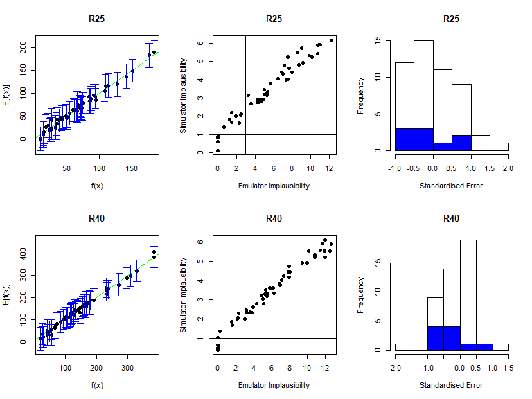
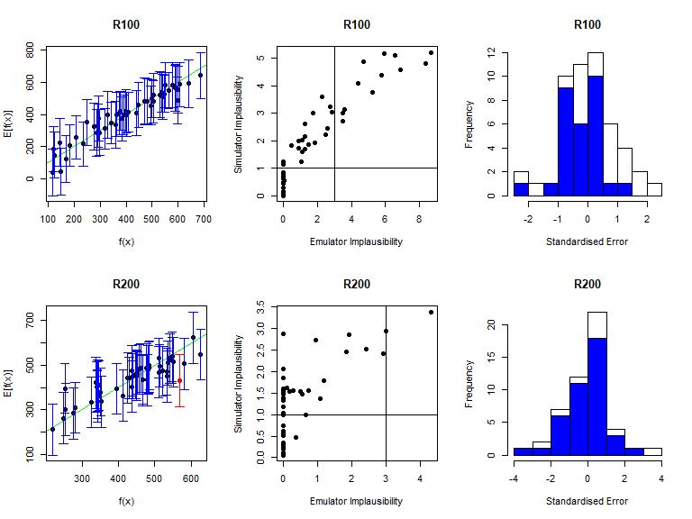
Note that by default validation_diagnostics groups the outputs in sets of three. Since here we have 8 outputs, we set the argument row to 2: this is not strictly necessary but improves the format of the grid of plots obtained. As in deterministic case, we can enlarge the $\sigma$ values of the mean emulators to obtain more conservative emulators, if needed. Based on the diagnostics above, all emulators perform quite well, so we won’t modify any $\sigma$ values here. In order to access a specific mean emulator, you can type ems$expectation$variable_name. For example, to double the $\sigma$ of the mean emulator for $I25$, you would type stoch_emulators$expectation$I25 <- stoch_emulators$expectation$I25$mult_sigma(2).

Note that the output vd of the validation_diagnostics function is a dataframe containing all parameter sets in the validation dataset that fail at least one of the three diagnostics. This dataframe can be used to automate the validation step of the history matching process. For example, one can consider the diagnostic check to be successful if vd contains at most $5\%$ of all points in the validation dataset. In this way, the user is not required to manually inspect each validation diagnostic for each emulator at each wave of the process.

It is possible to automate the validation process. If we have a list of trained emulators ems, we can start with an iterative process to ensure that emulators do not produce misclassifications:

check if there are misclassifications for each emulator (middle column diagnostic in plot above) with the function classification_diag;
in case of misclassifications, increase the sigma (say by 10%) and go to step 1.

The code below implements this approach:

for (j in 1:length(ems)) {
      misclass <- nrow(classification_diag(ems[[j]], targets, validation, plt = FALSE))
      while(misclass > 0) {
        ems[[j]] <- ems[[j]]$mult_sigma(1.1)
        misclass <- nrow(classification_diag(ems[[j]], targets, validation, plt = FALSE))
      }
}

The step above helps us ensure that our emulators are not overconfident and do not rule out parameter sets that give a match with the empirical data.

Once misclassifications have been eliminated, the second step is to ensure that the emulators’ predictions agree, within tolerance given by their uncertainty, with the simulator output. We can check how many validation points fail the first of the diagnostics (left column in plot above) with the function comparison_diag, and discard an emulator if it produces too many failures. The code below implements this, removing emulators for which more than 10% of validation points do not pass the first diagnostic:

bad.ems <- c()
for (j in 1:length(ems)) {
          bad.model <- nrow(comparison_diag(ems[[j]], targets, validation, plt = FALSE))
          if (bad.model > floor(nrow(validation)/10)) {
            bad.ems <- c(bad.ems, j)
   }
}
ems <- ems[!seq_along(ems) %in% bad.ems]

Note that the code provided above gives just an example of how one can automate the validation process and can be adjusted to produce a more or less conservative approach. Furthermore, it does not check for more subtle aspects, e.g. whether an emulator systematically underestimates/overestimates the corresponding model output. For this reason, even though automation can be a useful tool (e.g. if we are running several calibration processes and/or have a long list of targets), we should not think of it as a full replacement for a careful, in-depth inspection from an expert.