7 Emulator diagnostics

In this section we explore various diagnostic tests to evaluate the performance of the emulators and we learn how to address emulators that fail one or more of these diagnostics.

For a given set of emulators, we want to assess how accurately they reflect the model outputs over the input space. For a given validation set, we can ask the following questions:

• Allowing for uncertainty, does the emulator output accurately represent the equivalent model output?

• Does the emulator adequately classify parameter sets as implausible or non-implausible?

• What are the standardised errors of the emulator outputs in light of the model outputs?

The function validation_diagnostics provides us with three diagnostics, addressing the three questions above.

vd <- validation_diagnostics(ems_wave1$R200, validation = validation, 
                             targets = targets, plt=TRUE)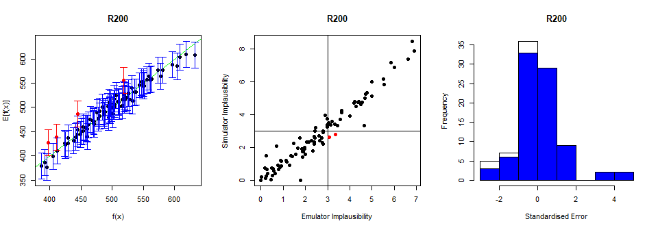

In the first column, the emulator expectation \(E[f(x)]\) is plotted against the model output \(f(x)\) for each validation point, providing the dots in the graph. The emulator uncertainty at each validation point is shown in the form of a vertical interval that goes from \(3\sigma\) below to \(3\sigma\) above the emulator expectation, where \(\sigma\) is the emulator variance at the considered point. An ‘ideal’ emulator would exactly reproduce the model results: this behaviour is represented by the green line \(f(x)=E[f(x)]\) (this is a diagonal line, visible here only in the bottom left and top right corners). Any parameter set whose emulated prediction lies more than \(3\sigma\) away from the model output is highlighted in red. Note that we do not need to have no red points for the test to be passed: since we are plotting \(3\sigma\) bounds, statistically speaking it is ok to have up to \(5\%\) of validation points in red (see Pukelsheim’s \(3\sigma\) rule).

The second column compares the emulator implausibility to the equivalent model implausibility (i.e. the implausibility calculated replacing the emulator output with the model output). There are three cases to consider:

• The emulator and model both classify a set as implausible or non-implausible (bottom-left and top-right quadrants). This is fine. Both are giving the same classification for the parameter set.

• The emulator classifies a set as non-implausible, while the model rules it out (top-left quadrant): this is also fine. The emulator should not be expected to shrink the parameter space as much as the model does, at least not on a single wave. Parameter sets classified in this way will survive this wave, but may be removed on subsequent waves as the emulators grow more accurate on a reduced parameter space.

• The emulator rules out a set, but the model does not (bottom-right quadrant): these are the problem sets, suggesting that the emulator is ruling out parts of the parameter space that it should not be ruling out.

As for the first test, we should be alarmed only if we spot a systematic problem, with \(5\%\) or more of the points in the bottom-right quadrant.

Finally, the third column gives the standardised errors of the emulator outputs in light of the model output: for each validation point, the difference between the emulator output and the model output is calculated, and then divided by the standard deviation \(\sigma\) of the emulator at the point. The general rule is that we want our standardised errors to be somewhat normally distributed around \(0\), with \(95\%\) of the probability mass between \(-3\) and \(3\). The blue bars indicate the distribution of the standardised errors when we restrict our attention only to parameter sets that produce outputs close to the targets. When looking at the standard errors plot, we should ask ourselves at least the following questions:

• Is more than \(5\%\) of the probability mass outside the interval \([-3,3]\)? If the answer is yes, this means that, even factoring in all the uncertainties in the emulator and in the observed data, the emulator output is too often far from the model output.

• Is \(95\%\) of the probability mass concentrated in a considerably smaller interval than \([-3,3]\) (say, for example, \([-0.5,0.5]\))? For this to happen, the emulator uncertainty must be quite large. In such case the emulator, being extremely cautious, will cut out a small part of the parameter space and we will end up needing many more waves of history matching than are necessary.

• Is the histogram skewing significantly in one direction or the other? If this is the case, the emulator tends to either overestimate or underestimate the model output.

The diagnostics above are not particularly bad, but we will try to modify our emulator to make it more conservative and avoid misclassifications in the bottom right quadrant (second column).

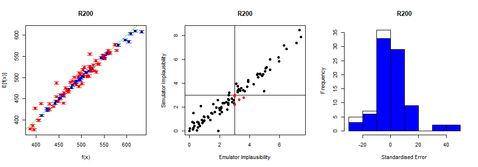
A way of improving the performance of an emulator is by changing its variance \(\sigma^2\). The lower the value of \(\sigma\), the more ‘certain’ the emulator will be. This means that when an emulator is a little too overconfident (as in our case above), we can try increasing \(\sigma\). Below we train a new emulator setting \(\sigma\) to be 2 times as much as its default value, through the method mult_sigma:

sigmadoubled_emulator <- ems_wave1$R200$mult_sigma(2)
vd <- validation_diagnostics(sigmadoubled_emulator, 
                             validation = validation, targets = targets, plt=TRUE)

A higher value of \(\sigma\) has therefore allowed us to build a more conservative emulator that performs better than before.

Task

Explore different values of \(\sigma\). What happens for very small/large values of \(\sigma\)?

Show: R tip

If em is an emulator, you can change its sigma by a factor x through the following line of code: em$mult_sigma(x).

Solution

Let us set \(\sigma\) to be ten times smaller than its default value:

tinysigma_emulator <- ems_wave1$R200$mult_sigma(0.1)
vd <- validation_diagnostics(tinysigma_emulator, validation = validation, 
                             targets = targets, plt=TRUE)

In this case we built a very overconfident emulator. This is shown by the very small uncertainty intervals in the first column: as a consequence many points are in red. Similarly, if we look at the third column we notice that the standardised errors are extremely large, well beyond the value of \(3\).

Let us now set \(\sigma\) to be ten times larger than its default value:

hugesigma_emulator <- ems_wave1$R200$mult_sigma(10)
vd <- validation_diagnostics(hugesigma_emulator, validation = validation, targets = targets,
                             plt=TRUE)

With this choice of \(\sigma\), we see that our emulator is extremely cautious. If we look at the plot in the middle, we see that now a lot of points in the validation set have an implausibility less or equal to \(3\). This implies that this emulator will reduce the input space slowly. As explained above, having consistent very small standardised errors is not positive: it implies that, even though we trained a regression hypersurface in order to catch the global behaviour of the output, the sigma is so large that the emulator is being dominated by the correlation structure. This means at best that we will have to do many more waves of history matching than are necessary, and at worst that our emulators won’t be able to reduce the non-implausible parameter space.

The above exploration highlights the importance of finding a value of \(\sigma\) that produces an emulator which on one hand is not overconfident and on the other is able to quickly reduce the input space.

It is possible to automate the validation process. If we have a list of trained emulators ems, we can start with an iterative process to ensure that emulators do not produce misclassifications:

1. check if there are misclassifications for each emulator (middle column diagnostic in plot above) with the function classification_diag;

2. in case of misclassifications, increase the sigma (say by 10%) and go to step 1.

The code below implements this approach:

for (j in 1:length(ems)) {
      misclass <- nrow(classification_diag(ems[[j]], targets, validation, plt = FALSE))
      while(misclass > 0) {
        ems[[j]] <- ems[[j]]$mult_sigma(1.1)
        misclass <- nrow(classification_diag(ems[[j]], targets, validation, plt = FALSE))
      }
}

The step above helps us ensure that our emulators are not overconfident and do not rule out parameter sets that give a match with the empirical data.

Once misclassifications have been eliminated, the second step is to ensure that the emulators’ predictions agree, within tolerance given by their uncertainty, with the simulator output. We can check how many validation points fail the first of the diagnostics (left column in plot above) with the function comparison_diag, and discard an emulator if it produces too many failures. The code below implements this, removing emulators for which more than 10% of validation points do not pass the first diagnostic:

bad.ems <- c()
for (j in 1:length(ems)) {
          bad.model <- nrow(comparison_diag(ems[[j]], targets, validation, plt = FALSE))
          if (bad.model > floor(nrow(validation)/10)) {
            bad.ems <- c(bad.ems, j)
   }
}
ems <- ems[!seq_along(ems) %in% bad.ems]

Note that the code provided above gives just an example of how one can automate the validation process and can be adjusted to produce a more or less conservative approach. Furthermore, it does not check for more subtle aspects, e.g. whether an emulator systematically underestimates/overestimates the corresponding model output. For this reason, even though automation can be a useful tool (e.g. if we are running several calibration processes and/or have a long list of targets), we should not think of it as a full replacement for a careful, in-depth inspection from an expert.