3 Introduction to the model

In this section we introduce the model that we will work with throughout our workshop.

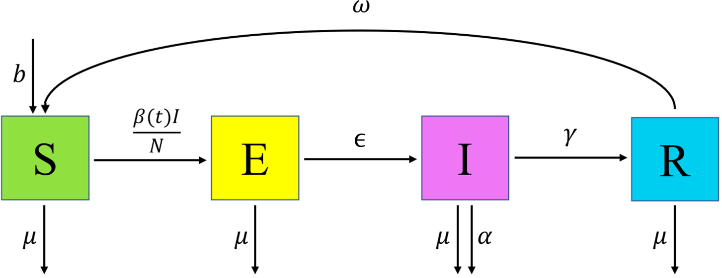
Figure 3.1: SEIRS Diagram

The model that we chose for demonstration purposes is a deterministic SEIRS model, described by the following differential equations: \[\begin{align} \frac{dS}{dt} &= b N - \frac{\beta(t)IS}{N} + \omega R -\mu S \\ \frac{dE}{dt} &= \frac{\beta(t)IS}{N} - \epsilon E - \mu E \\ \frac{dI}{dt} &= \epsilon E - \gamma I - (\mu + \alpha) I \\ \frac{dR}{dt} &= \gamma I - \omega R - \mu R \end{align}\] where \(N\) is the total population, varying over time, and the parameters are as follows:

• \(b\) is the birth rate,

• \(\mu\) is the rate of death from other causes,

• \(\beta(t)\) is the infection rate between each infectious and susceptible individual,

• \(\epsilon\) is the rate of becoming infectious after infection,

• \(\alpha\) is the rate of death from the disease,

• \(\gamma\) is the recovery rate and

• \(\omega\) is the rate at which immunity is lost following recovery.

The rate of infection between each infectious and susceptible individual \(\beta(t)\) is set to be a simple linear function interpolating between points, where the points in question are \(\beta(0)=\beta_1\), \(\beta(100) = \beta(180) = \beta_2\), \(\beta(270) = \beta_3\) and where \(\beta_2 < \beta_1 < \beta_3\). This choice was made to represent an infection rate that initially drops due to external (social) measures and then raises when a more infectious variant appears. Here \(t\) is taken to measure days. Below we show a graph of the infection rate over time when \(\beta_1=0.3, \beta_2=0.1\) and \(\beta_3=0.4\):

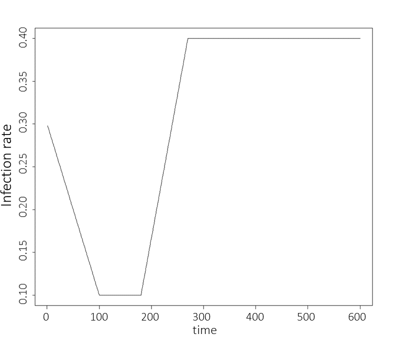
Figure 3.2: Infection rate graph

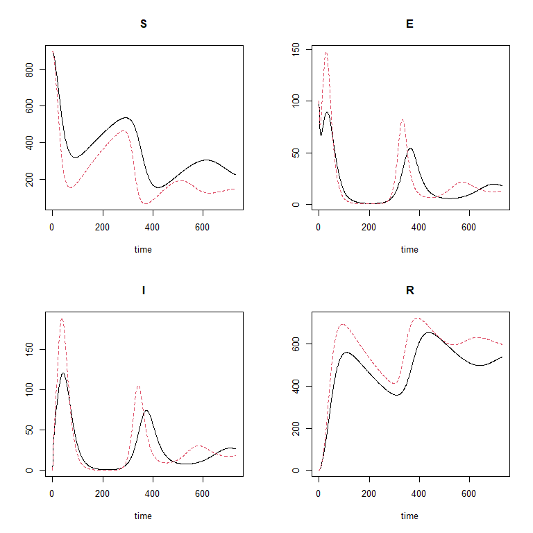
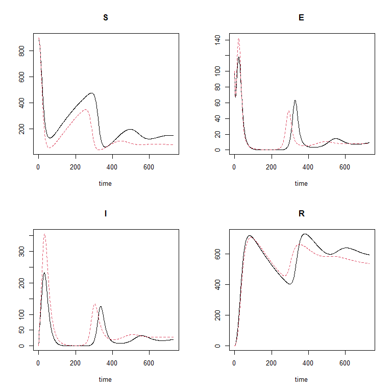
In order to obtain the solution of the differential equations for a given set of parameters, we will use a helper function, ode_results (which is defined in the R-script). The function assumes an initial population of 900 susceptible individuals, 100 exposed individuals, and no infectious or recovered individuals. Below we use ode_results with an example set of parameters and plot the model output over time.

example_params <- c(
  b = 1/(60*365),
  mu = 1/(76*365),
  beta1 = 0.2, beta2 = 0.1, beta3 = 0.3,
  epsilon = 0.13,
  alpha = 0.01,
  gamma = 0.08,
  omega = 0.003
)
solution <- ode_results(example_params)
par(mar = c(2, 2, 2, 2))
plot(solution)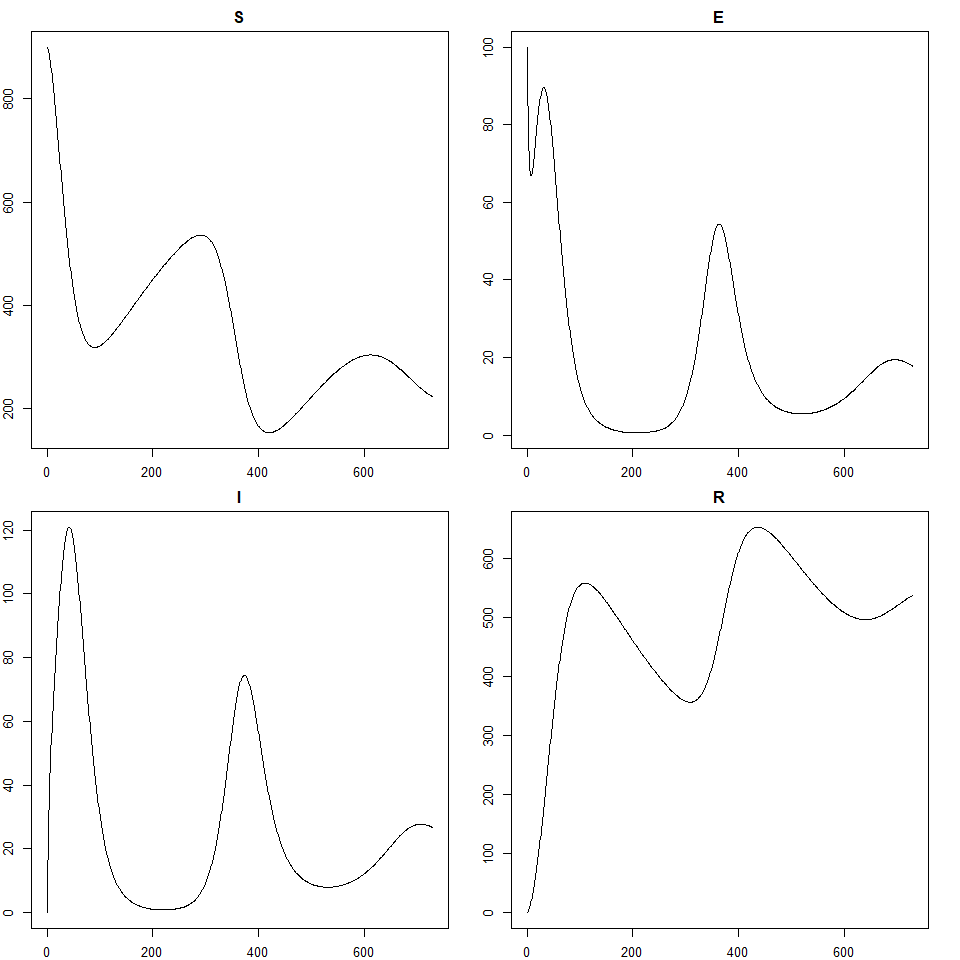

Task

Take some time to familiarise yourself with the model. Investigate how the plots change as you change the values of the parameters.

Show: R tip

Copy the code below, modify the value of (some) parameters and run it.

example_params <- c(
  b = 1/(60*365),
  mu = 1/(76*365),
  beta1 = 0.2, beta2 = 0.1, beta3 = 0.3,
  epsilon = 0.13,
  alpha = 0.01,
  gamma = 0.08,
  omega = 0.003
)
solution <- ode_results(example_params)
par(mar = c(2, 2, 2, 2))
plot(solution)

Solution

Let us see what happens when a higher force of infection is considered:

higher_foi_params <- c(
  b = 1/(60*365),
  mu = 1/(76*365),
  beta1 = 0.3, beta2 = 0.1, beta3 = 0.5,
  epsilon = 0.13,
  alpha = 0.01,
  gamma = 0.08,
  omega = 0.003
)
higher_foi_solution <- ode_results(higher_foi_params)
plot(solution, higher_foi_solution)

Here the black line shows the model output when it is run using the original parameters and the red dotted line when it is run using a higher force of infection. As expected, the number of susceptible individuals decreases, while the size of outbreaks increases.

Let us now also increase the rate of becoming infectious following infection \(\epsilon\):

higher_epsilon_params <- c(
  b = 1/(60*365),
  mu = 1/(76*365),
  beta1 = 0.3, beta2 = 0.1, beta3 = 0.5,
  epsilon = 0.21,
  alpha = 0.01,
  gamma = 0.08,
  omega = 0.003
)
higher_epsilon_solution <- ode_results(higher_epsilon_params)
plot(higher_foi_solution,higher_epsilon_solution)

Here the black line is the model output when the model is run with the previous parameter set, and the red dotted line is the model output when we also increase epsilon. We observe a decrease in the number of exposed individuals. Again, this is in agreement with our expectation: a higher rate of becoming infectious means that people leave the exposed compartmental to enter the infectious compartment faster than before.

Finally, what happens when a lower value of the recovery rate \(\gamma\) is used?

smaller_recovery_params <- c(
  b = 1/(60*365),
  mu = 1/(76*365),
  beta1 = 0.3, beta2 = 0.1, beta3 = 0.5,
  epsilon = 0.21,
  alpha = 0.01,
  gamma = 0.05,
  omega = 0.003
)
smaller_recovery_solution <- ode_results(smaller_recovery_params)
plot(higher_epsilon_solution, smaller_recovery_solution)

Here the black line is the model output when the model is run with the previous parameter set, and the red dotted line is the model output when we also decrease the recovery rate. Again, as one expects, this causes the number of susceptible individuals to decrease and the number of infectious individuals to increase, at least during the first peak.