6 Implausibility

In this section we focus on implausibility and its role in the history matching process. Once emulators are built, we want to use them to systematically explore the input space. For any chosen parameter set, the emulator provides us with an approximation of the corresponding model output. This value is what we need to assess the implausibility of the parameter set in question.

For a given model output and a given target, the implausibility measures the difference between the emulator output and the target, taking into account all sources of uncertainty. For a parameter set \(x\), the implausibility \(\text{Imp}(x)\) takes the following form in this tutorial:

\[\text{Imp}(x) = \frac{|f(x)-z|}{\sqrt{V_0 + V_c(x)+V_m}},\]

where \(f(x)\) is the emulator output, \(z\) the target, and

• \(V_0\) is the variance associated with the observation uncertainty (i.e. uncertainty in estimates from observed data);
• \(V_c(x)\) refers to the uncertainty one introduces when using the emulator output instead of the model output itself. Note that this term depends on \(x\), since the emulator is more/less certain about its predictions based on how close/far \(x\) is from training parameter sets.

The observation uncertainty \(V_0\) is represented by the ‘sigma’ values in the targets list, while \(V_c\) is the emulator variance, which we discussed in the previous section.

A very large value of \(\text{Imp}(x)\) means that we can be confident that the parameter set \(x\) does not provide a good match to the observed data, even factoring in the additional uncertainty that comes with the use of emulators. When \(\text{Imp}(x)\) is small, it could mean that the emulator output is very close to the model output or it could mean that the uncertainty in the denominator of \(\text{Imp}(x)\) is large. In the former case, the emulator retains the parameter set, since it is likely to give a good fit to the observation for that output. In the latter case, the emulator does not have enough information to rule the parameter set out and therefore keeps it to explore further in the next wave.

An important aspect to consider is the choice of cut-off for the implausibility measure. A rule of thumb follows Pukelsheim’s \(3\sigma\) rule, a very general result which states that for any continuous unimodal distribution \(95\%\) of the probability lies within \(3\) sigma of the mean, regardless of asymmetry (or skewness etc). Following this rule, we set the implausibility threshold to be \(3\): this means that a parameter \(x\) is classified as non-implausible only if its implausibility is below \(3\).

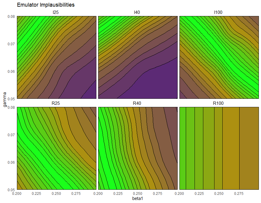
Given a set of emulators, we can plot their implausibility through the function emulator_plot by setting plot_type='imp'. Note that we also set cb=TRUE to ensure that the produced plots are colour blind friendly:

emulator_plot(ems_wave1, plot_type = 'imp', 
              targets = targets, params = c('beta1', 'gamma'), cb=TRUE)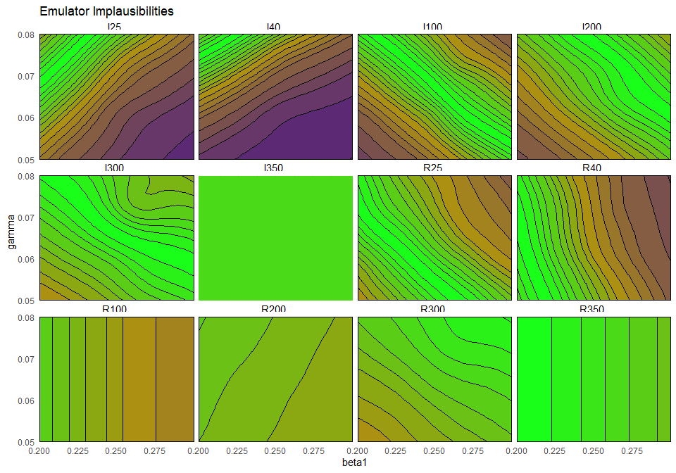

Each of the plots shows a 2D slice through the input space: for a chosen pair \((\bar\beta_1,\bar\gamma)\), the implausibility of the parameter set having \(\beta_1=\bar \beta_1\), \(\gamma=\bar \gamma\) and all other parameters set to their mid-range value is shown. Parameter sets with implausibility more than \(3\) are highly unlikely to give a good fit and will be discarded when forming the parameters sets for the next wave.

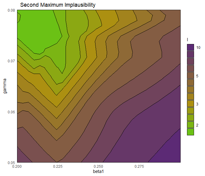
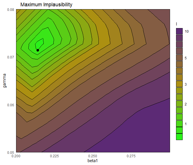
The plot just obtained is useful to get an overall idea of which emulators have higher/lower implausibility, but how do we measure overall implausibility? We want a single measure for the implausibility at a given parameter set, but for each emulator we obtain an individual value for \(I\). The simplest way to combine them is to consider maximum implausibility at each parameter set: \[\text{Imp}_M(x) = \max_{i=1,\dots,N}\text{Imp}_{i}(x),\] where \(\text{Imp}_i(x)\) is the implausibility at \(x\) coming from the \(i\)th emulator. Note that Pukelsheim’s rule applies for each emulator separately, but when we combine several emulators’ implausibilities together a threshold of \(3\) might be overly restrictive. For this reason, for large collections of emulators, it may be useful to replace the maximum implausibility with the second- or third-maximum implausibility. This also provides robustness to the failure of one or two of the emulators.

Task

Explore the functionalities of emulator_plot and produce a variety of implausibility plots. Here are a few suggestions:

• set plot_type to ‘imp’ to get implausibility plots or to ‘nimp’ to display the maximum implausibility plot;

• use the argument nth to obtain the second- or third- maximum implausibility plot;

• select a subset of all targets to pass to emulator_plot;

• change the value of the argument fixed_vals to decide where to slice the parameters that are not shown in the plots.

Solution

Let us start by visualising the maximum implausibility passing all emulators to emulator_plot and setting plot_type='nimp':

emulator_plot(ems_wave1, plot_type = 'nimp', targets = targets, 
              params = c('beta1', 'gamma'), cb=T)

This plot shows very high values of the implausibility for most points in the box. During the first few waves of history matching, one can consider second-maximum implausibility, rather than maximum implausibility. This means that instead of requiring the implausibility measure to be under the chosen threshold for all outputs, we allow (at most) one of them to be over it. This approach, which may result in less space cut out during the first few waves, has the advantage of being more conservative, reducing the risk that parts of the input space may be incorrectly cut. The more strict maximum implausibility measure can then be adopted in later waves, when the space to search is considerably smaller than the original input space, and the emulators less uncertain. To work with second-maximum implausibility we simply add nth=2 to the previous function call:

emulator_plot(ems_wave1, plot_type = 'nimp', targets = targets, 
              params = c('beta1', 'gamma'), cb=T, nth=2)

One of the advantages of history matching and emulation is that we are not obliged to emulate all outputs at each wave. This flexibility can be useful, for example, when the emulator for a given output does not perform well at a certain wave: we can simply exclude that output and emulate it in later waves. Another common situation where it may be useful to select a subset of emulators is when we have early outputs and late outputs, as in this workshop. It is often the case that later outputs have greater variability compared to earlier outputs, since they have more time to diverge. As a consequence, including emulators for later outputs in the first few waves may not be desirable: it would both increase the number of calculations to make (since we would train more emulators), and would probably contribute to a lesser extent to the reduction of the parameter space.

We can focus on early times outputs (e.g. up to \(t=100\)), and produce implausibility plots for them:

restricted_ems <- ems_wave1[c(1,2,3,7,8,9)]
emulator_plot(restricted_ems, plot_type = 'imp', targets = targets, 
              params = c('beta1', 'gamma'), cb=T)

Finally let us set the unshown parameters to be as in chosen_params (the parameter set used to define the targets, see Section 4):

emulator_plot(restricted_ems, plot_type = 'nimp', targets = targets[c(1,2,3,7,8,9)], 
              params = c('beta1', 'gamma'), 
              fixed_vals = chosen_params[!names(chosen_params) %in% c('beta1', 'gamma')], 
              cb=T)+geom_point(aes(x=0.214, y=1/14), size=3)

The plot shows what we expected: when \(\beta_1\) and \(\gamma\) are equal to their values in chosen_params, i.e. \(0.214\) and \(1/14\), the implausibility measure is well below the threshold \(3\) (cf. black point in the box).